the Creative Commons Attribution 4.0 License.
the Creative Commons Attribution 4.0 License.
 | 12 Apr 2022
Development of a forecast-oriented kilometre-resolution ocean–atmosphere coupled system for western Europe and sensitivity study for a severe weather situation
Joris Pianezze
Jonathan Beuvier
Cindy Lebeaupin Brossier
Guillaume Samson
Ghislain Faure
Gilles Garric
To improve high-resolution numerical environmental prediction, it is essential to represent ocean–atmosphere interactions properly, which is not the case in current operational regional forecasting systems used in western Europe. The objective of this paper is to present a new forecast-oriented coupled ocean–atmosphere system. This system uses the state-of-the-art numerical models AROME (cy43t2) and NEMO (v3.6) with a horizontal resolution of 2.5 km. The OASIS coupler (OASIS3MCT-4.0), implemented in the SurfEX surface scheme and in NEMO, is used to perform the communications between models. A sensitivity study of this system is carried out using 7 d simulations from 12 to 19 October 2018, characterized by extreme weather events (storms and heavy precipitation) in the area of interest. Comparisons with in situ and L3 satellite observations show that the fully coupled simulation reproduces the spatial and temporal evolution of the sea surface temperature and 10 m wind speed quantitatively well. Sensitivity analysis of ocean–atmosphere coupling shows that the use of an interactive and high-resolution sea surface temperature (SST), in contrast to actual numerical weather prediction (NWP) where SST is constant, modifies the atmospheric circulation and the location of heavy precipitation. Simulated oceanic fields show a large sensitivity to coupling when compared to the operational ocean forecast. The comparison to two distinct forced ocean simulations highlights that this sensitivity is mainly controlled by the change in the atmospheric model used to drive NEMO (AROME vs. IFS operational forecast), and less by the interactive air–sea exchanges. In particular, the oceanic boundary layer depths can vary by more than 40 % locally, between the two ocean-only experiments. This impact is amplified by the interactive coupling and is attributed to positive feedback between sea surface cooling and evaporation.


Ocean–atmosphere feedbacks occur over a wide range of spatial and temporal scales. They play a critical role in the evolution of climate (Intergovernmental Panel on Climate Change, 2014) but also in the evolution of smaller-spatial- and smaller-temporal-scale phenomena like tropical cyclones (Bender and Ginis, 2000; Smith et al., 2009; Jullien et al., 2014); mid-latitude storms (Mogensen et al., 2018; Bouin and Lebeaupin Brossier, 2020b), sometimes leading to heavy-precipitation events as for instance in the Mediterranean region (Rainaud et al., 2017; Meroni et al., 2018); dense water formation (Carniel et al., 2016; Lebeaupin Brossier et al., 2017); and ocean dynamics in particular in response to strong wind (e.g. Pullen et al., 2006; Small et al., 2012; Renault et al., 2019b; Jullien et al., 2020). It is therefore essential to represent them in numerical models to correctly predict atmosphere and ocean dynamics for climate, environmental or weather applications. Since the 1960s, global coupled ocean–atmosphere systems have indeed developed and been used to investigate the future climate change (e.g. Meehl, 1990; Eyring et al., 2016) and, later on, served for seasonal forecasts (e.g. Stockdale et al., 1998). With the increase in high-performance-computer (HPC) resources (Shukla et al., 2010), many regional coupled research systems have been developed since the 2000s' (e.g. Bao et al., 2000; Chen et al., 2010; Warner et al., 2010; Voldoire et al., 2017), and it is now possible to reach coupled ocean–atmosphere simulation in dedicated regions with a horizontal resolution of only a few kilometres for both components (e.g. Pellerin et al., 2004; Small et al., 2011; Grifoll et al., 2016; Ličer et al., 2016; Rainaud et al., 2017; Pianezze et al., 2018; Vilibić et al., 2018; Lewis et al., 2019; Thompson et al., 2021). At that resolution, (i) an atmospheric model explicitly represents the deep convection, the major gravity waves and the main interactions with orography (Weusthoff et al., 2010), and (ii) oceanic model is classified as eddy-rich resolution solving major baroclinic oceanic eddies (Hewitt et al., 2020).
Among these new kilometric ocean–atmosphere coupled systems, only a few aim at operational oceanography purposes or numerical weather prediction (NWP) applications, and even fewer are run operationally despite spread motivations and common interests (Brassington et al., 2015; Pullen et al., 2017). The main obstacles to this remain in particular the computing costs of an atmospheric model for operational oceanography and, in general, a lower expertise on one or the other of the components and the absence of coupled initialization strategy and dedicated validation tools.
To step forward, Météo-France and Mercator Ocean International (MOI) recently joined their development efforts to build a new forecast-oriented coupled system based on two models used for operational purposes, which is presented in this paper. This new coupled system is an extension and update of the ocean–atmosphere coupled system developed by Rainaud et al. (2017) and Lebeaupin Brossier et al. (2017), which involves the regional non-hydrostatic NWP system of Météo-France, AROME and NEMO, the ocean model operated routinely by MOI for ocean forecasting. This new configuration covers western Europe and the western part of North Africa and includes the western Mediterranean Sea (up to Sicily eastwards) and also part of the northeast Atlantic Ocean, the English Channel, and the North and Irish seas (Fig. 1). This region is characterized by fine-scale ocean structures: estuaries and regions of freshwater influence related to large river plums (e.g. Simpson et al., 1993; Brenon and Le Hir, 1999; Estournel et al., 2001; Bergeron, 2004); thermal fronts notably in the French Atlantic continental shelf area (Yelekçi et al., 2017) and in particular the Ushant front of tidal origin (Chevallier et al., 2014; Redelsperger et al., 2019), or also the North Balearic Front in the western Mediterranean Sea (García et al., 1994); slope current, wind-driven circulation and mesoscale eddies in the Bay of Biscay (van Aken, 2002; Le Boyer et al., 2013); gyres in the Alboran Sea (Viúdez et al., 1998); meanders of the Algerian Current and eddies (Millot et al., 1990; Millot and Taupier-Letage, 2005); and shelf circulation, cyclonic gyre, ocean deep convective area and Northern Current in the Gulf of Lions (e.g. Millot, 1991; Echevin et al., 2003; Testor et al., 2018; Carret et al., 2019). Furthermore, it is also frequently affected by several kinds of natural hazards of weather origin: strong wind related to storm, cyclogenesis (Trigo et al., 2002; Trigo, 2006) with an explosive development for some cases (Liberato et al., 2013) or even tropical-like characteristics (namely medicanes, Miglietta and Rotunno, 2019), sometimes interacting locally with the coast and/or orography (like mistral and tramontane, Bastin et al., 2006; Obermann et al., 2018); thunderstorms (Taszarek et al., 2019) including Mediterranean heavy-precipitation events with floods (Ducrocq et al., 2016); and heat waves (De Bono et al., 2004; Darmaraki et al., 2019; Ma et al., 2020), in which ocean–atmosphere interactions play a significant role. Better representing the air–sea feedback that occurs at fine scale in this area is therefore relevant, and developing a dedicated ocean–atmosphere coupled prediction system now appears essential to improve the high-resolution regional forecasts on both sides.
In that way, our common scientific objectives in this development between Météo-France and MOI are (1) to share and improve knowledge about fine-scale ocean–atmosphere interactions in this wider region; (2) to be able to provide high-resolution and consistent atmosphere and ocean forecasts over western Europe and notably the entire French coastal area, including the Corsican coasts; and (3) to prepare a coupled initialization strategy also able to ensure consistency with the large-scale driver models used at the boundaries.
The new coupled system and the coupling strategy are presented in Sect. 2. Sections 3 and 4 respectively present the experimental design and the coupled and forced simulation results, as the coupling impacts for both atmospheric and oceanic forecasts. Finally, conclusions and perspectives are given in Sect. 5.
In this section the models and the coupling strategy used in this new coupled system are presented. The simulation domain is presented in Fig. 1, with comparison to the actual operational regional domains for both AROME(-France) and NEMO(-NEATL36). The atmospheric and oceanic domains follow different projections inherited from the “best” options for each of the two models, and they thus induce a specific treatment of the masked areas that is described in Sect. 2.3.
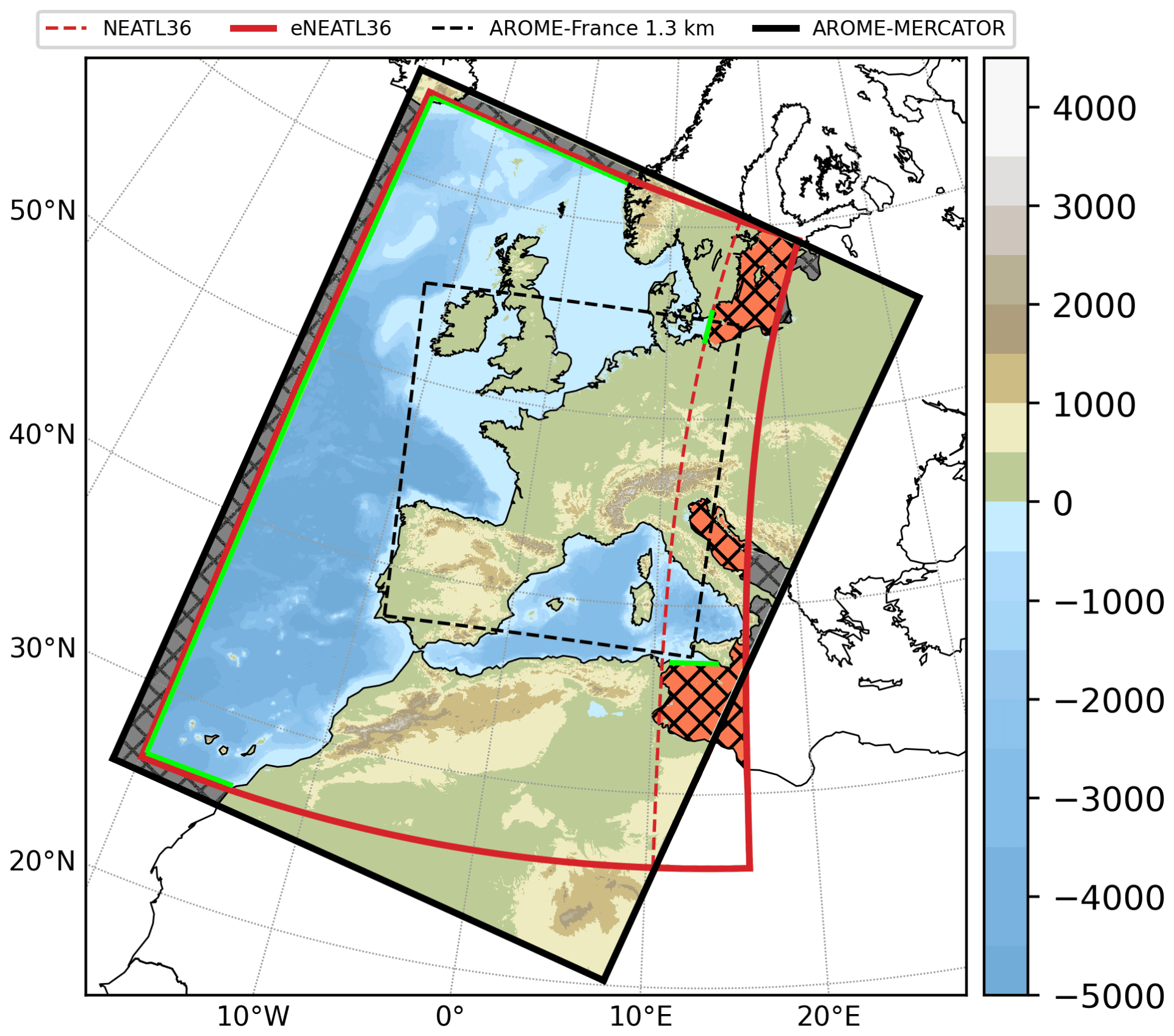
Figure 1Simulation domain illustrated by the bathymetry (m) in NEMO (in blue) and by the orography (m) of the AROME model (in green-brown colours). The lines indicate the extension of the NEMO-eNEATL36 configuration (red) and of the AROME-Mercator domain (black); the green lines highlight the open boundaries in the oceanic model. For AROME-Mercator, the grey and orange marine zones are always uncoupled (constant initial SST and null current are used; see text). For eNEATL36, the orange marine zones are not solved in the regional oceanic simulations. The dashed lines indicate the boundaries of the actual operational configurations of AROME (AROME-France, 1.3 km resolution, in black) and NEMO over the Iberia–Biscay–Ireland (IBI) region (NEATL36, 1/36∘ resolution, in red).
2.1 Oceanic model
The oceanic model used in this coupled system is based on version 3.6 of the Nucleus for European Modelling of the Ocean model (NEMO, Madec et al., 2017). It is a state-of-the-art primitive-equation, split-explicit, free-surface oceanic model. It was built from the operational Iberia–Biscay–Ireland (IBI) configuration (originally on the NEATL36 grid, Maraldi et al., 2013; Sotillo et al., 2015; Gutcknecht et al., 2019; Sotillo et al., 2021), spatially extended eastwards in the Mediterranean Sea (see the eNEATL36 grid in Fig. 1). The meridian boundary in the IBI operational configuration located between the Gulf of Genoa, Corsica, Sardinia and Tunisia has been moved to a zonal boundary between Tunisia and Sicily; thus this new regional configuration now covers the entire Tyrrhenian Sea. The horizontal resolution is 1/36∘ with 1294×1894 horizontal grid points, and the vertical grid contains 50 stretched z levels. The vertical level thickness is 0.5 m at surface and around 450 m for the last levels (i.e. at 5700 m depth).
The temporal scheme for both tracer and momentum is a leapfrog scheme associated with a Robert–Asselin filter to prevent model instabilities (Leclair and Madec, 2009). The free surface is explicit with time splitting, with a baroclinic time step of 150 s and a barotropic time step 30 times smaller. Momentum advection is computed based on the vector invariant form while the total variation diminishing (TVD) scheme is used for tracer advection in order to conserve energy and enstrophy (Barnier et al., 2006). The generic length scale (GLS) scheme is used in that configuration, which is based on two prognostic equations: one for the turbulent kinetic energy and another for the generic length scale (Umlauf and Burchard, 2003, 2005).
Open boundary conditions (OBCs) are based on the 2D characteristic method (Blayo and Debreu, 2005). The atmospheric pressure component is added, hypothesizing pure isostatic response at open boundaries (inverse barometer approximation). As in the operational IBI configuration (Sotillo et al., 2015, 2021), river freshwater inputs are imposed partly as daily OBC in the domain locations for 33 main rivers and partly as a climatological coastal runoff to close the water budget from land. For the 33 main rivers explicitly considered, flow-rate data are based on a combination of daily observations, simulated data (from SMHI E-HYPE hydrological model) and climatology (monthly climatological data from GRDC and French “Banque Hydro” dataset). The tidal forcing is prescribed from the FES2014 dataset (Carrere et al., 2015) and applied as an unstructured boundary in the NEMO domain: 11 tidal harmonics (M2, S2, N2, K1, O1, Q1, M4, K2, P1, Mf, Mm) are used. Solar penetration is parameterized according to a five-band exponential scheme (considering the UV radiations) function of surface chlorophyll concentrations, using a monthly climatological version of the Copernicus Marine Environment Monitoring Service (or Copernicus Marine Service) (CMEMS) European Space Agency Climate Change Initiative (ESA-CCI) product covering the northeast Atlantic area (OCEANCOLOUR_ATL_CHL_L4_REP_OBSERVATIONS_009_091, Colella et al., 2020).
In that new configuration, version 2.0 of the eXtensible Markup Language XML Input/Output Server (XIOS, Meurdesoif, 2013) is used to manage NEMO output files.
The model is initialized by fields from the operational IBI configuration at 1/36∘ (IBI36, Sotillo et al., 2021) on the common domain (see Fig. 1) and from the global CMEMS configuration at 1/12∘ (GLO12, Lellouche et al., 2018) in the Tyrrhenian Sea and forced at the OBC (green lines in Fig. 1) with daily analyses from this CMEMS GLO12 configuration.
2.2 Atmospheric and surface models
The atmospheric model used in this new coupled system is cycle 43 (cy43t2) of the non-hydrostatic Application de la Recherche à l'Opérationnel à Méso-Échelle (AROME) NWP regional model (Seity et al., 2011; Brousseau et al., 2016). The AROME physical configuration used here is close to the one operationally used at Météo-France but covers a wider area (than the AROME-France NWP 1.3 km resolution model) around western Europe (Fig. 1), with a 2.5 km resolution, and is run here without data assimilation. This AROME domain, with a Lambert conformal projection, has been specifically defined and oriented in order to cover the eNEATL36 domain, but with a slightly wider extent notably to avoid some spurious atmospheric boundary effects that affect the ocean component.
In more detail, AROME has 1285×1789 horizontal grid points and a vertical grid of 90 hybrid η levels with a first-level thickness of almost 5 m. The advection scheme in AROME is semi-Lagrangian, and the temporal scheme is semi-implicit with a time step of 50 s. The 1.5-order turbulent kinetic energy scheme from Cuxart et al. (2000) is used. The surface current acts in two ways on turbulence by using the relative winds, i.e. the difference between the near-surface winds and the surface oceanic currents, instead of absolute winds (i) in the computation of air–sea fluxes and (ii) in the tri-diagonal problem associated with the discretization of the vertical turbulent viscosity because of the implicit treatment of the bottom boundary condition in the atmospheric model. Only the first effect was included in the former AROME–NEMO couplings (Rainaud et al., 2017; Lebeaupin Brossier et al., 2017; Sauvage et al., 2021). For the purpose of this study, the full current-feedback (CFB) effect has been added in the turbulent scheme of AROME, following Renault et al. (2019a) and based on the exact same developments as previously done in the MESO-NH model (Bouin and Lebeaupin Brossier, 2020a).
Thanks to its 2.5 km horizontal resolution, the deep convection is explicitly resolved while the shallow convection is parameterized with the eddy diffusion Kain–Fritsch (EDKF, Kain and Fritsch, 1990) scheme. The ICE3 one-moment microphysical scheme of Pinty and Jabouille (1998) is used to compute the evolution of five hydrometeor species (rain, snow, graupel, cloud ice and cloud liquid water). Radiative transfer is based on the Fouquart and Bonnel (1980) scheme for short-wave radiation and the Rapid Radiative Transfer Model (RRTM, Mlawer et al., 1997) for long-wave radiation.
The surface exchanges are computed by the SURFace EXternalisé (SURFEX) surface model (Masson et al., 2013) considering four different surface types: land, towns, sea and inland waters (lakes and rivers). Output fluxes are weight-averaged inside each grid box according to the fraction of each respective tile, before being provided to the atmospheric model at every time step. Exchanges over land are computed using the ISBA (interactions between soil, biosphere and atmosphere) parametrization (Noilhan and Planton, 1989). The formulation from Charnock (1955) is used for inland waters, whereas the town energy balance (TEB) scheme is activated over urban surfaces (Masson, 2000). For the sea surface, the albedo is computed following the Taylor et al. (1996) scheme, and sea surface fluxes are computed with the COARE3.0 parametrization (Fairall et al., 2003).
Like when run operationally, AROME in this configuration can be initialized and forced at its lateral boundaries by operational global analyses and/or forecasts from Action de Recherche Petite Echelle Grande Echelle (ARPEGE; Courtier et al., 1991) or Integrated Forecasting System (IFS; ECMWF, 2020). No lateral boundary condition is applied in SurfEx, which is initialized over continental surfaces with the ARPEGE surface analysis.
2.3 Coupling strategy
Communications between AROME/SurfEx and NEMO models are performed with the Ocean–Atmosphere–Sea Ice–Soil coupler (OASIS3-MCT_4.0, Valcke, 2013; Craig et al., 2017). OASIS3-MCT is a library allowing synchronized exchanges of coupling information between different numerical models. OASIS calls were inserted in SurfEx sources by Voldoire et al. (2017), allowing the atmosphere–ocean coupling between AROME/SurfEx and NEMO.
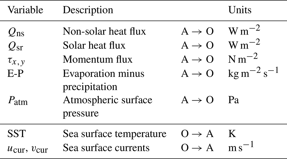
During the coupled simulation, AROME-SurfEx sends the net non-solar heat flux, the two components of the wind stress and the net freshwater flux computed for the sea tile only to NEMO, and they are then imposed at the surface boundary condition of NEMO (Table 1). The solar heat flux is also sent to NEMO and is used to calculate the penetrative radiation in the ocean. Contrary to Rainaud et al. (2017), Lebeaupin Brossier et al. (2017) and also Arnold et al. (2021), the possibility of exchanging atmospheric surface pressure was implemented in this study and is also exchanged interactively during the coupled simulation for the inverse barometer approximation. In return, NEMO sends the sea surface temperature and the sea surface current components to AROME-SurfEx, and they then enter in the sea surface turbulent flux computation and in the atmospheric turbulence scheme.
The remapping files needed to interpolate fields between NEMO and AROME-SurfEx with a distance-weighted nearest-neighbour interpolation method using four neighbours are created offline using OASIS tools. Figure 1 presents the masked parts of each domain. The orange areas in Fig. 1 correspond to areas where the regional NEMO-eNEATL36 does not resolve the ocean (ocean in these areas is resolved in the global GLO12 configuration, which gives information through the open boundaries, highlighted in green in Fig. 1). In AROME, the masked area corresponds to the same unsolved areas of the regional NEMO configuration plus the northern, western and southern extensions. Where the ocean is masked for being outside the regional NEMO domain (orange and grey hashed areas in Fig. 1), AROME uses a SST constant in time and equal to the one used at the initial time, and the surface currents taken are always equal to zero.
Table 1Variables exchanged between NEMO (O) and AROME/SurfEx (A) via the OASIS3-MCT coupler.
3.1 Case study: storms and high precipitation (12–19 October 2018)
The sensitivity of this coupled system is carried out through 7 d simulations of a case study from 12 to 19 October 2018. During these 7 d western Europe experienced a severe weather sequence (see Fig. 2) with a mid-latitude storm (Callum), two (ex-)tropical cyclones (Leslie and Michael) and a Mediterranean heavy-precipitation event (Aude HPE case).
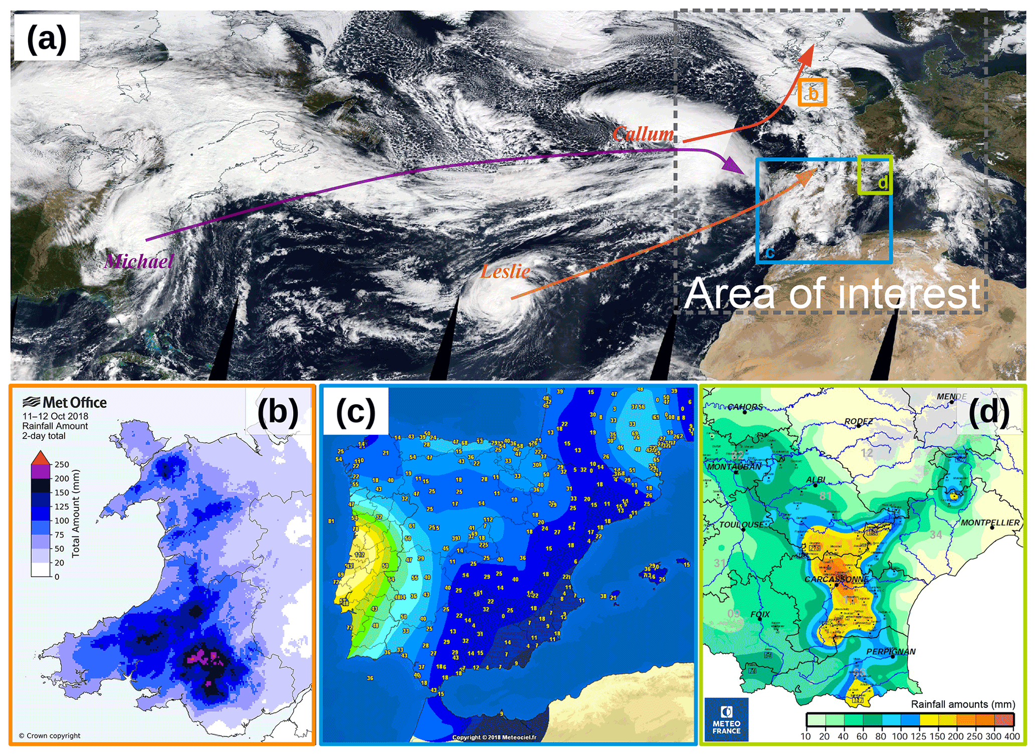
Figure 2Illustrations of the case study. (a) True colour image of Terra/MODIS (source: https://worldview.earthdata.nasa.gov/, last access: 7 April 2022) on 11 October 2018 over the North Atlantic Ocean showing the storm Callum and the hurricanes Leslie and Michael (arrows depict their trajectories towards the area of interest); (b) rainfall totals (mm) from 11 to 12 October 2018 over Wales (Callum's impacts, Fig. 64 from Kendon et al., 2019, source: MetOffice); (c) wind gust observations (km h−1) over the Iberian Peninsula on 13 October 2018 around 23:00 UTC (Leslie's landfall, source: https://www.meteociel.fr/, last access: 7 April 2022); (d) rainfall amounts (mm) between 06:00 UTC on 14 October and 06:00 UTC on 15 October 2018 over the French Languedoc region (Aude event, source: Météo-France – edited 19 February 2019).
In more detail, storm Callum was named by Met Éireann on 10 October when it was forecast to affect the British Islands and more particularly Ireland and Wales. The storm deepened over the Atlantic Ocean on 11 October, reaching a minimum pressure depth of 938 hPa. On 12 October, strong wind affected Ireland and northwestern Wales, with gusts up to 140 km h−1 at Capel Curig. Heavy rainfall also occurred over Wales (Fig. 2b), in particular inland due to an orographic enhancement, with up to 219 mm in 36 h recorded at Libanus (Powys), making Callum one of the most severe rainfall events across Wales in the last 50 years (Kendon et al., 2019). Storm Callum indeed had strong impacts due to flooding, also because the wind peak coincided with high spring tides and led to large waves, with some coastal flooding, largely enhanced by the heavy rainfall.
Hurricane Leslie was a large, long-lived and very erratic tropical cyclone over the Atlantic. Followed by the National Hurricane Center (NHC) since 23 September (Pasch and Roberts, 2019), it struck the Iberian Peninsula on the evening of 13 October. For the first time on record, a tropical storm warning was issued for Madeira. In fact, after a stationary position in the eastern Atlantic at the beginning of October, Leslie started moving and intensifying under a favourable environment with slightly warmer water, thus re-attaining hurricane status on 10 October. Leslie reached its peak intensity with maximum sustained winds of 150 km h−1 and a minimum central pressure of 968 hPa on 00:00 UTC 12 October, about 1000 km south-southwest of the Azores. While then re-weakening, Leslie raced east-northeastwards, accelerated by the mid-latitude westerlies, and passed about 320 km north-northwest of Madeira at 06:00 UTC on 13 October. At 18:00 UTC, Leslie became a strong extratropical cyclone, at about 190 km west-northwest of Lisbon. Leslie's extratropical remnant finally made landfall close to Figueira da Foz (Coimbra District) just after 21:00 UTC with wind gusts above 110 km h−1 (Fig. 2c), heavy rains and strong waves. Spain was also affected by strong wind with up to 96 km h−1 in Zamora (Castile and Leòn). Leslie's centre became ill-defined after it moved over the Bay of Biscay on 14 October. At the same time, it induced favourable and steady conditions for heavy rainfall in the western Mediterranean, with the Leslie remnant acting as a large trough and generating a southerly flow.
As described in Caumont et al. (2021) and Mandement and Caumont (2021), in the night of 14 to 15 October 2018 the Languedoc region in the south of France was indeed affected by heavy rainfall caused by a regenerative multi-cellular convective system organized along a convergence line between the moist southerly low-level flow and a quasi-stationary cold front over southwestern France along a mean sea level pressure (MSLP) trough that linked Leslie to a low located over Ireland. During the evening and night of 14 to 15 October, a low rapidly deepened around the cold front and induced a strong convective activity over the Catalan Sea, between the Balearic Islands and Valencia region. The most intense rainfall occurred between 19:00 UTC 14 October and 07:00 UTC 15 October. The Météo-France quantitative precipitation estimation gives a maximum 24 h accumulated rainfall total of 342 mm close to Trèbes (Aude, Fig. 2d). Intense rainfall mainly occurred in less than 12 h, leading to flash floods in particular in Villegailhenc (Aude) and causing 15 fatalities.
Some days after, the extratropical cyclone Michael emerged into the Atlantic around 06:00 UTC on 12 October after passing near Norfolk (Virginia, US). Michael re-obtained hurricane-force winds on 13 October in the Atlantic waters south of Nova Scotia and Newfoundland and then quickly travelled within westerlies to the northeastern Atlantic on 14 October. The cyclone turned sharply southeastward and later southward around the northeastern edge of the subtropical ridge, weakening slightly as it approached the Iberian Peninsula. Michael dissipated by 00:00 UTC on 16 October, while it was located just west of northern Portugal, and just after Leslie's remnant was absorbed into Michael's remnant, following a brief Fujiwhara (1921) interaction.
This 7 d period chosen as the weather situation encountered is known to foster large air–sea interactions, but also because both ocean and weather forecasts may exhibit a larger sensitivity to coupling in such conditions. This is analysed through different simulations in the coupled and forced modes that are described in the following section.
3.2 Experiments
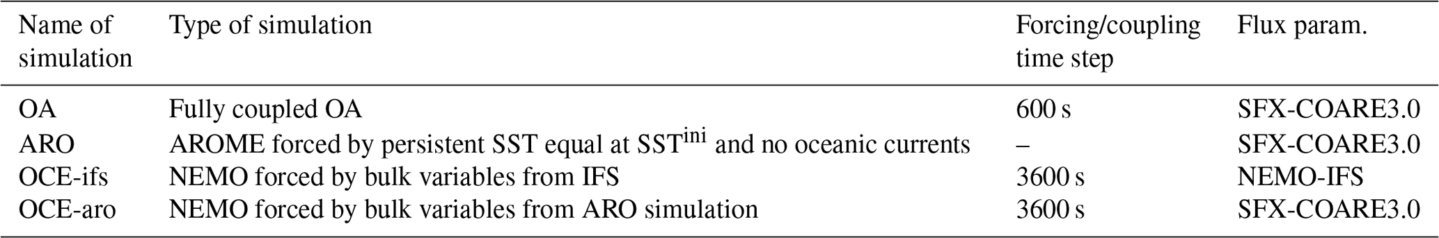
To evaluate the ocean–atmosphere coupling impact on the atmospheric and oceanic forecasts, four experiments were performed and are detailed below and in Table 2.
The ocean–atmosphere (OA) experiment is the ocean–atmosphere coupled forecast over 7 d, starting on 12 October 2018, 00:00 UTC. The initial atmospheric conditions come from the global IFS analysis of 12 October 2018, 00:00 UTC and the lateral atmospheric forcing comes every 6 h from the global IFS forecast starting on 12 October 2018, 00:00 UTC. The initial ocean fields come from the combination, as described in 2.1, of the CMEMS IBI and GLO12 analyses (3D daily fields of 11 October) and OBC for the 7 d come from the CMEMS GLO12 daily analyses. The ocean–atmosphere coupling period is set to 600 s; i.e. the fields are exchanged every 4 NEMO time steps and 12 AROME time steps.
The reference experiment for atmospheric forecast (ARO) is similar to the OA experiment except that, as uncoupled, (i) the SST is kept persistent in time and (ii) sea surface currents are not taken into account. Note that this ARO experiment is equivalent to one operational deterministic execution of AROME at Météo-France (called AROME-IFS), but with two adaptations. First, the lateral atmospheric condition frequency is changed to 6 h in order to be able to run over a 7 d period (against 42 to 48 h for AROME operational forecasts). This was mandatory due to less frequent forecast outputs available for the longest-term ranges of IFS. And secondly, for consistency with OA, the initial SST field is the combination of the GLO12 and IBI SST fields (instead of the ARPEGE SST analysis for AROME-IFS). Thus, comparing ARO with OA allows us to evaluate the ocean–atmosphere coupling impact, i.e. the effect of an interactive evolution of SST and the impact of taking currents into account, on the weather forecast.
Two ocean-only experiments were also run. OCE-ifs is the standard ocean simulation close to the operational mode of IBI: the initial conditions consist in the combination of the CMEMS IBI and GLO12 analyses (3D daily fields of 11 October) and OBC for the 7 d come from the CMEMS GLO12 daily analyses (similarly to the ocean component of OA). The atmospheric forcing uses the bulk variables from IFS (2 m air temperature, 2 m humidity, 10 m wind components, rainfall, mean sea level pressure, short-wave and long-wave solar fluxes) and the IFS bulk parametrization (ECMWF, 2020) available in the NEMO surface scheme (meaning the SST evolution and sea surface currents are taken into account to compute the air–sea exchanges). OCE-aro is an intermediate simulation using the ARO (AROME) bulk variables as atmospheric forcing (the same bulk variables as for IFS are used except for the wind speed which is taken at 5 m, the height of the first vertical level of AROME) and the COARE3.0 sea surface turbulent flux parametrization (Fairall et al., 2003) through SURFEX offline. Comparing OCE-aro with OA on the one hand and OCE-aro with OCE-ifs on the other permits as to disentangle the ocean–atmosphere coupling effect on the ocean forecast from the impact of the atmospheric forcing change.
4.1 Oceanic forecast
This section presents the evaluation of the coupled OA simulation for ocean surface and upper-layer parameters and the impacts of both the high-resolution atmospheric forcing and ocean–atmosphere coupling on the oceanic forecasts.
4.1.1 Sea surface temperature
At the initial state of OA (as for all the simulations), a latitudinal SST gradient is visible, from 7 ∘C in the northwest to more than 24 ∘C in the southwest part of the domain and in the Mediterranean Sea (Fig. 3a). Small-scale structures in SST are also visible and are related to the presence of mesoscale oceanic eddies, resolved at that 1/36∘ horizontal resolution (or partly resolved in the Mediterranean part). After 1 (Fig. 3b) and 3 (Fig. 3c) simulated days, the signatures of the Callum, Leslie and Mickael storms are visible with an associated sea surface cooling of up to 2.5 ∘C persisting during the 7 simulated days (Fig. 3d). This cooling is mainly due to oceanic vertical mixing processes enhanced by the strong wind produced by these storms. At the end of the 7 simulated days, the average temperature over the domain is 0.6 ∘C colder than initially, with local differences varying up to 35 % of the initial SST (cooler or warmer depending on the location). The maximum differences are located in the areas of influence of the storms (Atlantic Ocean).
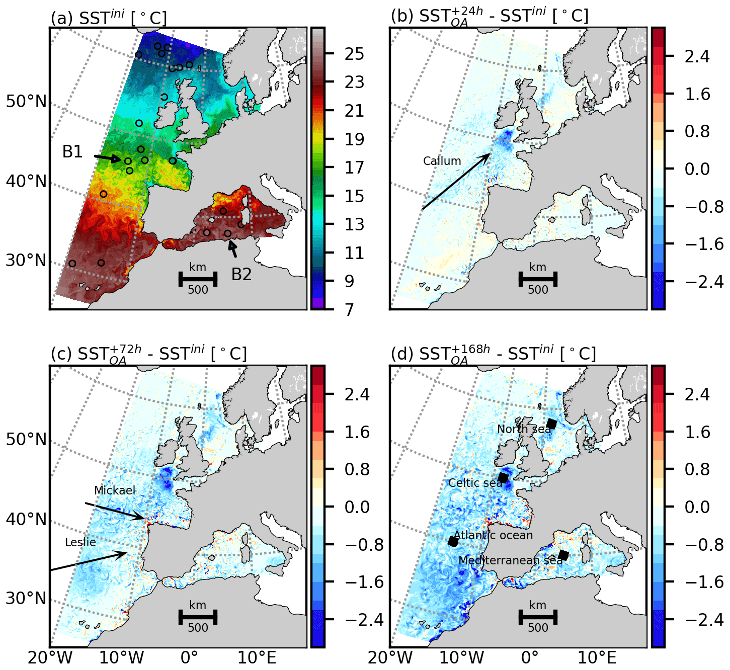
Figure 3Initial SST (12 October 2018, 00:00 UTC) (a) and evolution of the SST (∘C) after 1 d (b), 3 d (c) and 7 d (d) in the coupled simulation (OA; Table 2). In (a), the colour circles represent the SST measured by drifting buoys at that time ; B1 and B2 labels indicate the location of the two drifting buoys used in Fig. 5. Black squares in (d) correspond to four extracted areas used for analysis in the next subsections.
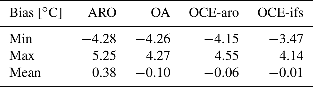
In Fig. 4 and Table 3, the sea surface temperature after 168 h (7 d) for all simulations (Table 2) is compared to satellite observations coming from the CMEMS portal (SST_EUR_L3S_NRT_OBSERVATIONS_010_009_a, Orain et al., 2021). This L3 SST is obtained from several satellite sensors which are combined together and interpolated on a regular 0.02∘ grid and is available every day with daily average. In order to be able to compare the simulated and observed SST fields, it is necessary to interpolate the simulated SST on the satellite observation grid, taking into account the masked areas related to the presence of clouds and therefore where no satellite data are available (white areas in Fig. 4a, b, c, d). Whether at the beginning or at the end of the simulation, the simulated SST values are close to the observed SST with a mean bias of less than 0.4 ∘C. The maximum differences are present in the ARO simulation where the SST is persistent (the case in AROME operational configuration used at Météo-France) (Fig. 4a). Its average is about +0.38 ∘C over the whole domain and varies from −4.28 to +5.25 ∘C locally. Unlike the ARO simulation, the other simulated temperatures have a lower average negative bias below −0.1 ∘C (Fig. 4b, c, d). Among these three simulations, the SST values simulated by the OA (Fig. 4b) and OCE-aro (Fig. 4c) simulations are very close, with biases equal to −0.1 and −0.06 ∘C respectively and values varying locally by about ± 4.3 ∘C. We can note that the intense cooling located in the Celtic Sea already identified in Fig. 3 is stronger than the observed one (Fig. 4b, c). This cooling related to the Callum passage persists throughout the coupled OA and OCE-aro simulations but not in the OCE-ifs simulation, which has a more important restratification (Fig. 4d). In the rest of the paper, we will show that this cooling is attributed to the simulated AROME surface winds (used to compute the surface turbulent fluxes in the OA and OCE-aro simulations), which are stronger than the surface winds simulated by IFS (used to compute the surface turbulent fluxes in the OCE-ifs simulation), inducing more intense oceanic mixing in OA and OCE-aro simulations than in the OCE-ifs one. The SST closest to the observations is the SST simulated by the OCE-ifs simulation, which has an average bias of −0.01 ∘C varying from −3.47 to +4.14 locally.
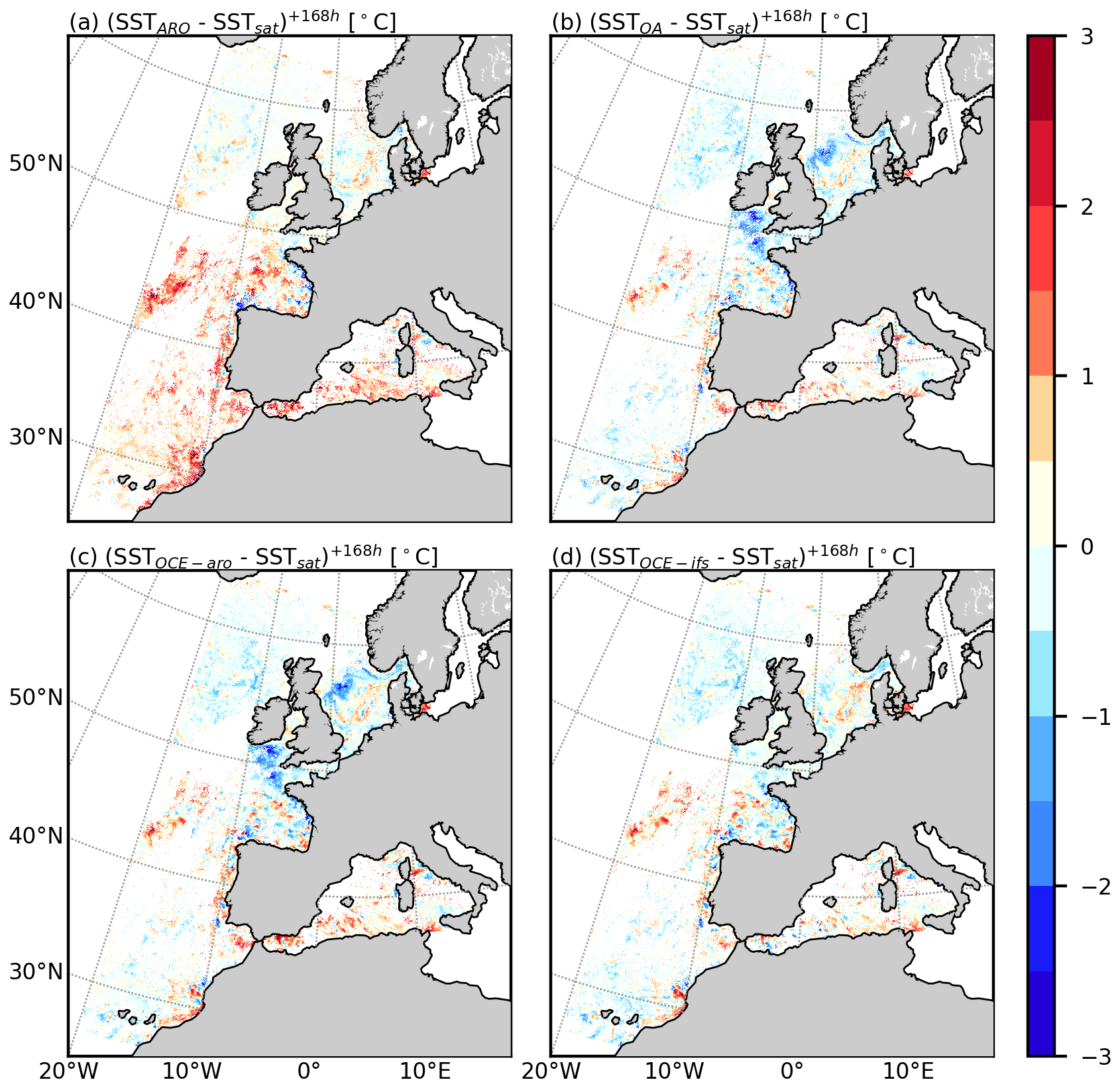
Figure 4Comparison with L3 satellite SST observations at the end of the simulation (19 October 2018, 00:00 UTC) : differences (∘C) with (a) ARO SST, (b) OA simulated SST, (c) OCE-aro simulated SST and (d) OCE-ifs simulated SST.
Table 3Minimum, maximum and mean SST bias (∘C) values against L3 SST observations at the end of the simulated period (19 October 2018, 00:00 UTC, i.e. +168 h) for each experiment (note that ARO SST is constant since 12 October 2018, 00:00 UTC). This table is complementary to Fig. 4.
Temporal evolution of simulated sea surface temperature is also compared to in situ observations (drifting buoys) available on the Coriolis project portal (http://www.coriolis.eu.org, last access: 7 April 2022) in Fig. 5 (the locations of the observations used for the comparison are shown in Fig. 3a). Among the full observational dataset, we select only data which have almost full time series during the 7 simulated days (33 drifting buoys), and with an hourly period (see B1 and B2 examples in Fig. 5a, b). Despite this selection, the high density of drifting buoy observations allows us to evaluate the simulated SST over the entire domain. For all the buoys represented in Fig. 3a, statistics for all the experiments (Table 2) are computed and are summarized in the Taylor diagram in Fig. 5c. The SST simulated by the ARO simulation is the furthest from the observations, with a deviation from the observed SST that increases during the simulation (Fig. 5a and b) and a mean bias around 0.4∘C (Fig. 5c). This important bias is clearly visible in Fig. 5a and b. For other simulations (OA, OCE-aro and OCE-ifs; Table 2), the mean bias is quite similar around 0.04 ∘C and the standard deviation is 0.2 ∘C, but scores show a large variability. The correlation is 0.4 on average. The examples of B1 and B2 illustrate the good behaviour of all simulations in representing the weekly surface cooling. The rapid and intense SST variations are also reproduced, as visible for B1 (Fig. 5a), related to the storm Callum, or for the diurnal cycle seen at B2 (Fig. 5b), on 12 and 18 October for example in OA, however with differences in terms of intensity with respect to observations. In spite of local differences, the OA, OCE-aro and OCE-ifs simulations thus accurately reproduce the mean gradient, mesoscale structures and evolution of SST during the 7 simulated days.
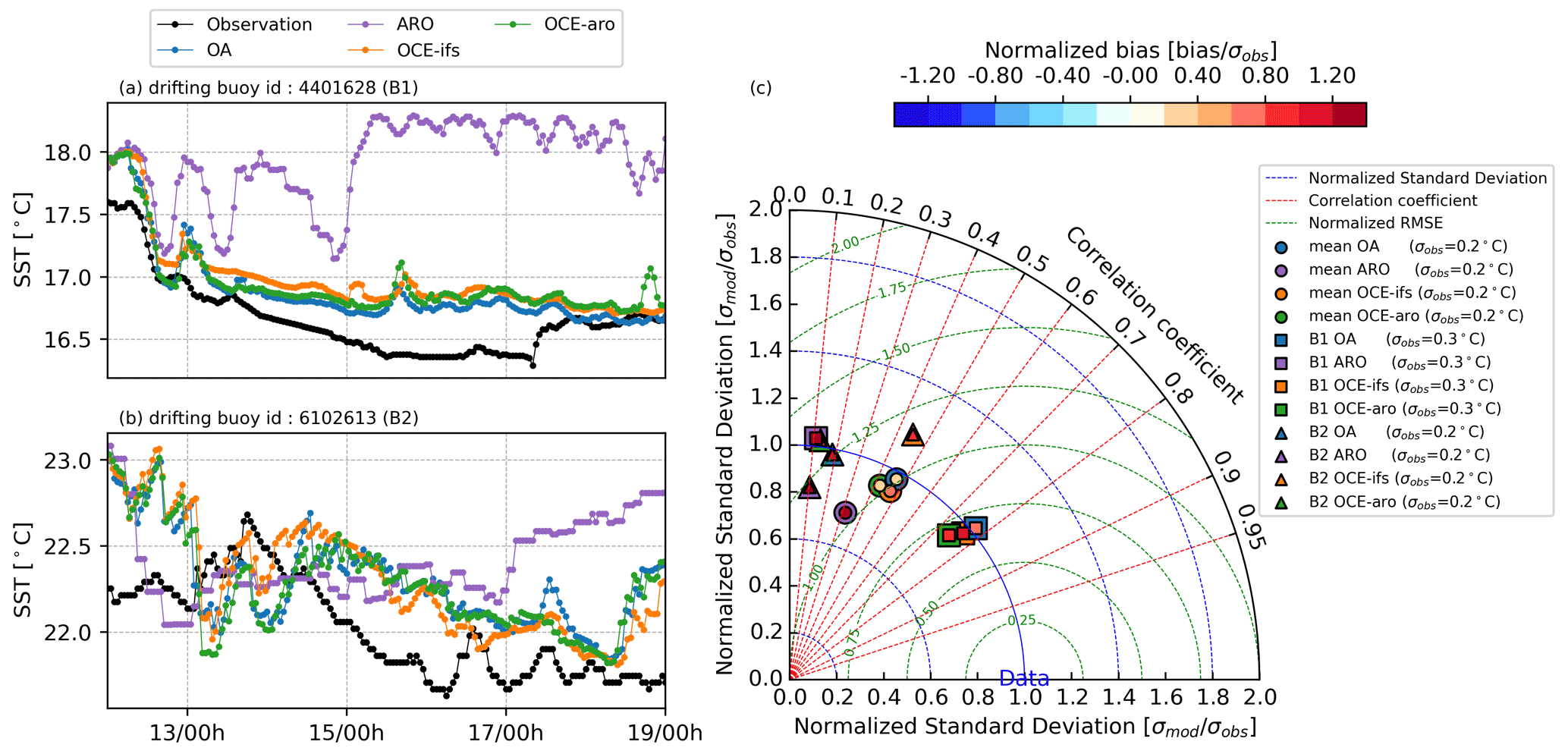
Figure 5Temporal evolution of sea surface temperature observed and simulated at the location of the buoys B1 (a) and B2 (b). (c) Taylor diagram made from comparison with 33 selected buoys visible in Fig. 3a. Mean statistics for the 33 selected buoys are represented in circles, statistics for buoy B1 only in squares and for buoy B2 only in triangles. The inner colour indicates the normalized bias. The external colour indicates the experiment: blue for OA, purple for ARO, orange for OCE-ifs and green for OCE-aro.
In order to further evaluate the numerical experiments, we chose to focus on some dedicated locations, where intense air–sea interactions are expected. For that, we define four boxes of 50 km×50 km, and their locations are visible in Fig. 3d (black squares).
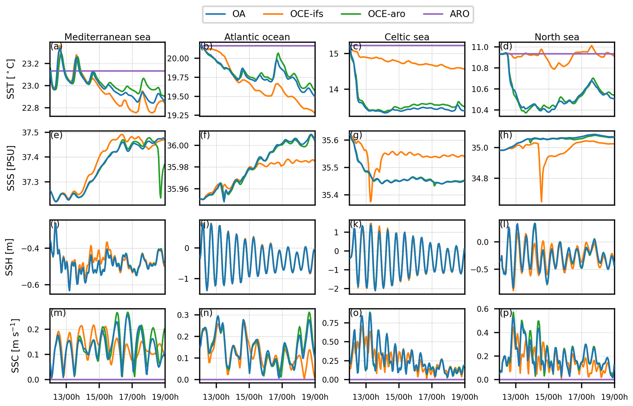
Temporal evolution of sea surface temperature in these four boxes is presented in Fig. 6a, b, c, d. As discussed in the previous paragraph, the simulated SST decreases during the 7 simulated days in OA as in OCE-aro and OCE-ifs, with diurnal variations visible in the Mediterranean Sea at the beginning of the simulated period. In the Celtic and North seas, the sea surface temperature decreases by more than 1.5 and 0.5 ∘C in less than 1 d respectively for OA and OCE-aro simulations. In OCE-ifs (Fig. 6d), no sea surface cooling is visible in the North Sea, and cooling of 0.3 ∘C in 1 d is visible in the Celtic Sea, 5 times lower than sea surface cooling in the OA and OCE-aro simulations (Fig. 6b, c). Changing the atmospheric forcing of NEMO between IFS and AROME drastically modifies the oceanic response, with a more intense sea surface cooling for simulations using AROME (see OA in blue and OCE-aro in green in Fig. 6c, d). Thus, the effect of changing the atmospheric model to force NEMO is larger than the effect of an interactive coupling on the simulated surface fields, in particular for SST and sea surface salinity (SSS) forecast. However, the effect of the ocean–atmosphere coupling on the SST and SSS also induces a feedback, leading to a more important cooling of the surface waters in coupled (OA) than in forced (OCE-aro) simulations. This sea surface cooling enhancement with coupling is in fact related to a lower non-solar net heat flux in OA (not shown), meaning a larger heat loss at night (and a lower diurnal heating) for ocean in OA than in OCE-aro. In fact, the surface cooling rapidly changes the atmospheric low-level environment and stability (without significant difference in the wind speed (and wind stress)). In particular, the coupled simulation represents an amplification loop, as the 2 m specific humidity is progressively lower in OA (than in OCE-aro/ARO). This enhances evaporation and thus slightly amplifies the surface cooling. We can note that this effect of ocean–atmosphere coupling is visible for all boxes after 3 simulated days, and differences increase until the end of the simulation (see Fig. 6a, b, c, d). Using a persistent SST for extreme events (ARO simulation) can lead to large errors (more than 0.5 ∘C in 2 d) as is shown in Fig. 6a, b, c.
4.1.2 Sea surface dynamics, salinity and ocean mixed layer
As for the temporal evolution of sea surface temperature, the sea surface salinity (SSS), sea surface height (SSH) and sea surface currents (SSCs) are extracted in the four locations (Fig. 3d, black squares) and are presented in Fig. 6e to p.
In addition to SSS variations due to tide, the SSS time series show a global increase in the Mediterranean, Atlantic Ocean and North Sea (Fig. 6e, f, h). It reaches about +0.04 PSU d−1 over the 7 simulated days in the Mediterranean and is 2 times lower for the two others (i.e. Atlantic Ocean and North Sea boxes). The strong evaporation fluxes linked to the presence of high winds are responsible for these increases (not shown). Only the Celtic Sea shows a decrease in SSS of −0.15 PSU in the first 36 simulated hours (Fig. 6g). This can be explained by the intense oceanic mixing associated with strong winds, which tends to mix less salty water to the surface, while the precipitation associated with the passage of Callum does not contribute significantly to the decrease in SSS in this area (not shown). The SSS simulated by OA and OCE-aro simulations has similar variabilities, and the effect of OA coupling is not visible. However, differences of the order of −0.1 PSU are visible between these two simulations and the OCE-ifs one. This can be explained by different freshwater fluxes (evaporation minus precipitation) between the AROME and IFS simulations.
With respect to SSH variations (Fig. 6i, j, k, l), they are strongest in the Celtic Sea where the tidal amplitude is higher. The amplitude of these variations reaches 4 m and decreases over the 7 d, in relation to the decrease in the tidal coefficient from 95 on 12 October to 30 on 17 October (values for Brest harbour). In the Atlantic Ocean, the variation in SSH is also important with an amplitude of 1 m, while it is weaker in the North Sea, due to a smaller amplitude of the tidal harmonics in this area, leading also to a more variable signal related to interactions between these harmonics. In the Mediterranean Sea, the SSH variations have the smallest amplitude (≈0.2 m), which are in fact mainly related to the presence of oceanic eddies. The main signal being due to the tidal oscillations, differences between the three simulations are relatively small or even indistinguishable, meaning that the effect of the choice of the atmospheric forcing model or OA coupling on SSH is an order of magnitude smaller than the tidal forcing.
Figure 6m, n, o, p show the impact of atmospheric forcing on the sea surface currents (SSC) in the four extracted areas. Note that in the coupled experiment (OA; Table 2), the sea surface currents are also exchanged. The spatial and temporal evolution of these currents is important during the 7 simulated days. Their intensity is maximum in the Channel, reaching more than 2 m s−1 locally, due to tidal currents (not shown). SSCs are maximum in the Celtic and North seas, reaching more than 0.5 m s−1 with intensities that vary with respect to the tides. For the Atlantic Ocean and Mediterranean Sea boxes, SSC intensity is less important but can reach up to 0.25 m s−1. SSCs are on average less intense in the OCE-ifs simulation than in the OA and OCE-aro simulations, which is explained by weaker winds in IFS than in AROME (Sect. 4.2). Also, for the Mediterranean box, on 14–15 October, the SSC is stronger in OCE-ifs than in OA and OCE-aro during that period (Fig. 6m). The impact of OA coupling on SSC is not significantly important.
The evolution of the ocean mixed layer is analysed more finely thanks to temporal evolution of temperature vertical profiles (Fig.7). Black lines in Fig. 7 correspond to ocean mixed layer depth (MLD). To compute this mixed layer depth, the potential density field is used: for each grid point, the value at 10 m depth is taken as a reference, and the mixed layer depth is obtained when the vertical difference is higher than 0.01 kg m−3 (pycnocline depth). At the beginning of the OA, OCE-aro and OCE-ifs simulations (Table 2), the MLD is around 40 m in the Atlantic Ocean, the Channel and the North Sea. In the Mediterranean, the MLD is thinner, around 20–30 m, corresponding to typical MLD values for late summer (D'Ortenzio et al., 2005). The MLD is stable in the Mediterranean and deepens slightly in the Atlantic, from 40 to 50 m during the 7 d simulated for all simulations. At these locations, differences between the simulations are also quite small (Fig. 7b, c, e, f) or only related to differences in the mixing, mainly due to the wind forcing (Fig. 7b, e). The strongest MLD variations are located in the northwestern part of the domain, in the Celtic Sea (Fig. 7g, h, i) and North Sea (Fig. 7j, k, l) boxes, where a significant deepening of the MLD is visible during the first simulated days for OA and OCE-aro simulations. This MLD deepening reaches 35 m in the first simulated days in the North Sea and up to 65 m in the Celtic Sea. Storm Callum and its associated high turbulent fluxes are responsible for this strong MLD deepening. After the passage of Callum, a slow restratification is simulated in the Celtic Sea from 14 October, which is also present but less visible in the North Sea. These changes are not only located in the near-surface waters (where it exceeds −2 ∘C) but also deeper, and even below the mixed layer depth (black line in Fig. 7g, j). For the Celtic Sea and North Sea boxes, differences between the OA simulation and the OCE-ifs simulation are large (± 2.5 ∘C corresponding to a mixing-induced dipole with cooling near the surface and warming near the thermocline, Fig. 7h, k) and much higher than the differences between the OA and the OCE-aro simulations (Fig. 7i, l). More generally for the four boxes, differences are larger when comparing OCE-ifs to OA than when comparing OA and OCE-aro. This illustrates that the effect of changing the atmospheric forcing has a larger effect on ocean surface and also vertical profiles than changing from a forced to a coupled simulation. OCE-ifs and OCE-aro have been compared to the available in situ profile measurements (Argo floats, CTD profiles, mooring, gliders and drifting buoys, from the CORA 5.2 database, Szekely et al., 2019) for the ocean mixed layer (OML) temperature (i.e. around 13 m depth) through root mean square errors (RMSEs, Fig. 8) to further examine the mixed layer representation. It shows in fact that the two ocean-only simulations have quite similar skill scores on average over the domain and along the simulation period, with very slightly lower RMSE for OCE-ifs than for OCE-aro (Fig. 8b), but some large improvements are found locally when using AROME forcing, notably along the Cornwall coast in the Celtic Sea (Fig. 8a).
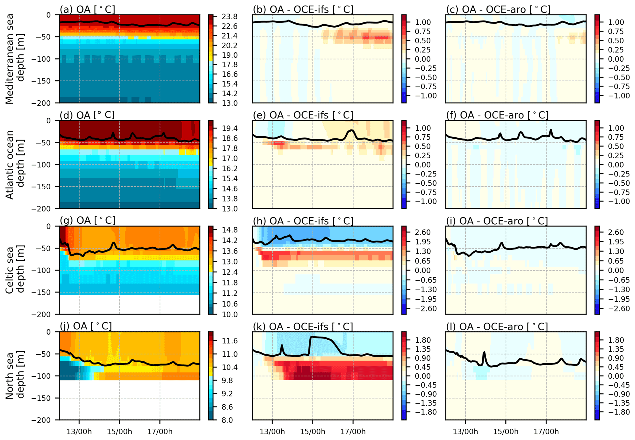
Figure 7Temporal evolution of the mean vertical temperature profiles in the four zones (see Fig. 3d) simulated by the coupled (OA) simulation (a, d, g, j) and differences with the two forced ocean simulations (OA-OCE-ifs in b, e, h, k and OA-OCE-aro in c, f, i, l). The black lines delimit the averaged MLD of OA (a, d, g, j), OCE-ifs (b, e, h, k) and OCE-aro (c, f, i, l).
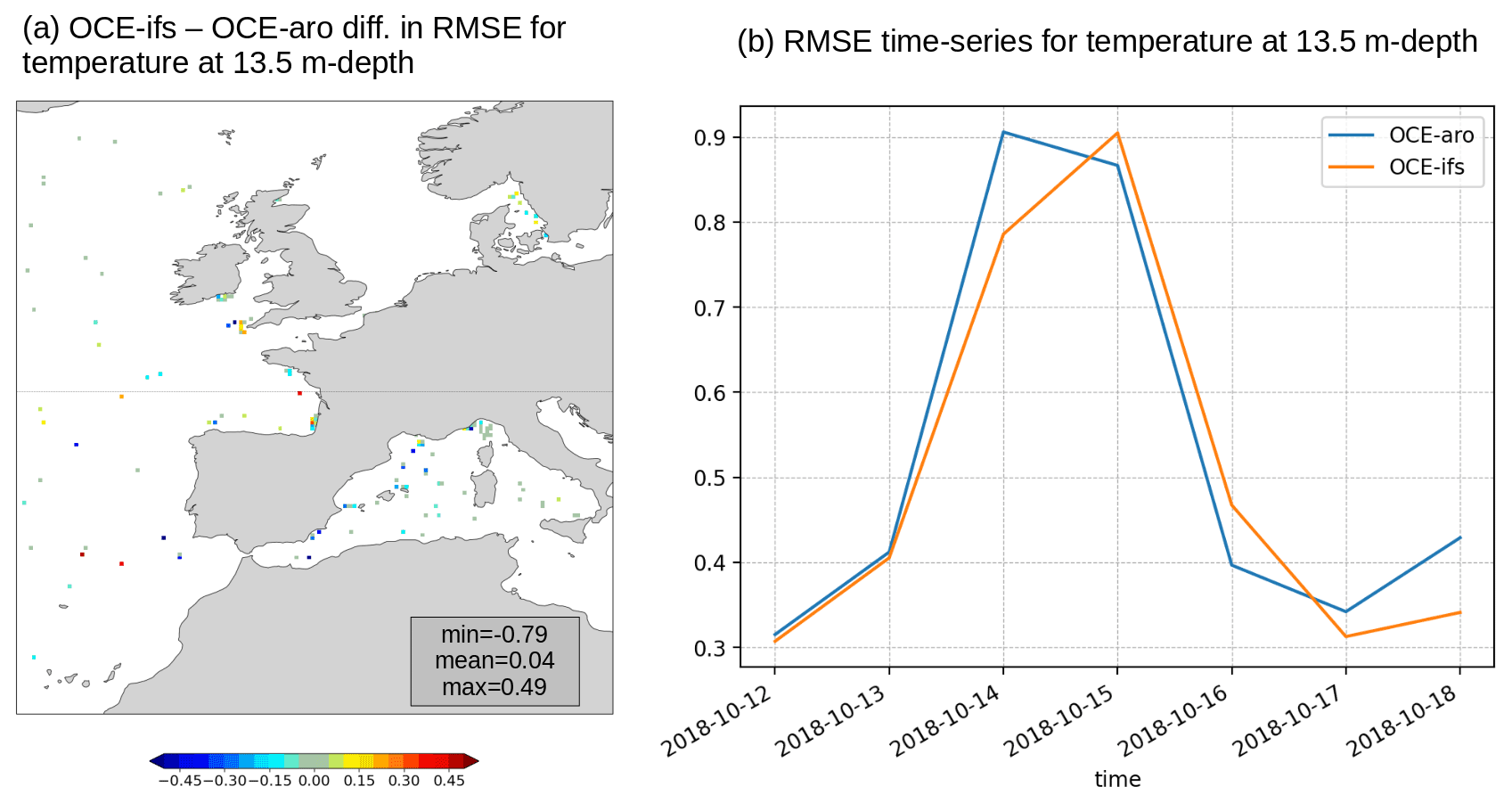
Figure 8Forecast error for temperature at vertical level 10 (around 13.5 m depth), expressed as a RMSE in degrees Celsius: (a) difference between OCE-ifs errors and OCE-aro errors at observation points, during the 7 simulated days (blue dot means lower RMSE in OCE-ifs); (b) time series of the daily error, averaged over all observations available for each day, for OCE-ifs and OCE-aro.
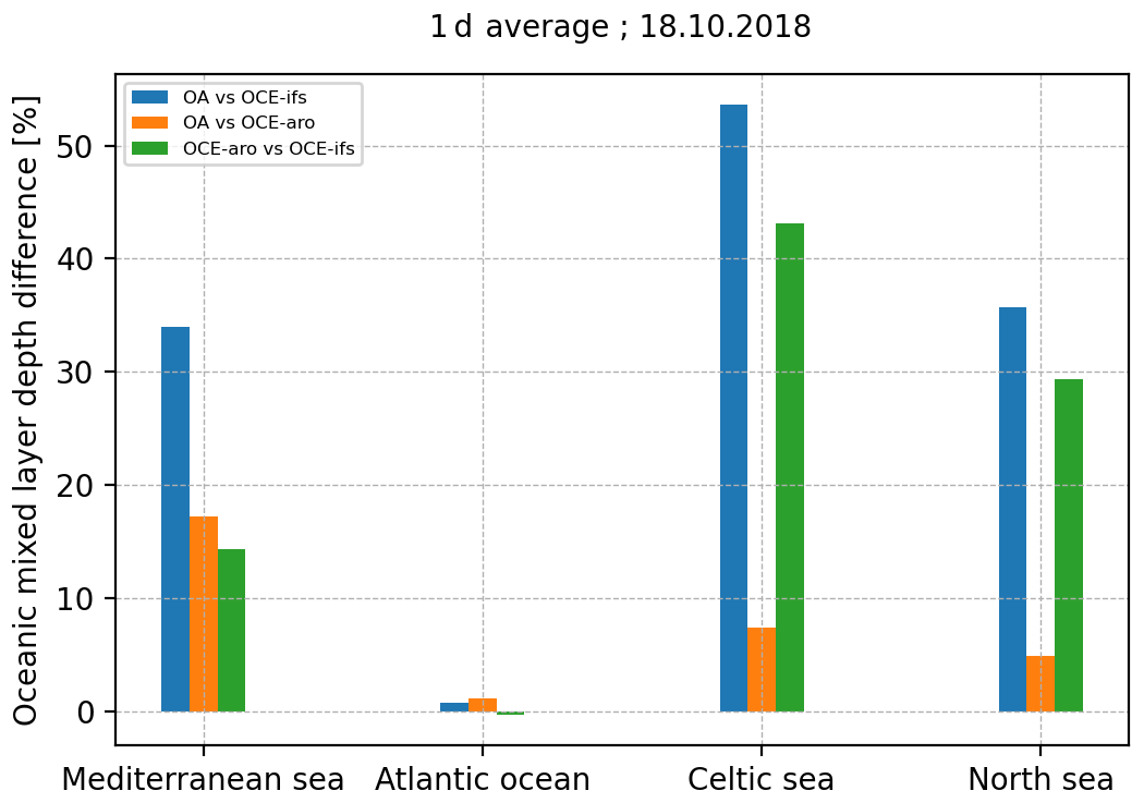
Differences between daily-averaged (last simulated day) ocean mixed layer depth (MLD) simulated by the three simulations (OA, OCE-ifs and OCE-aro) are represented in Fig. 9. The highest daily-averaged MLD values are found in the northwesternmost part of the domain, around 100 m deep, up to 150 m locally, and in the Celtic Sea (80–100 m) (Fig. 9a). The smallest values (<30 m) are found in the coastal areas (in relation with lower SSS values in the river plumes) and in the Mediterranean Sea.

Figure 9Daily-averaged oceanic mixed layer depth (m) simulated by OA simulation on the last day of simulation (a) and differences (in metres) with OCE-ifs- and OCE-aro-forced simulations (b, c).
Maximum differences between OA and OCE-ifs are localized around the British Islands and can reach ± 50 m. Here again, differences between OA and OCE-aro are smaller, even if located in the same areas (Fig. 9c). When computing the relative differences between OA and OCE-ifs (blue bars in Fig. 10), they exceed more than 50 % in the Celtic Sea and 30 % in the North and Mediterranean seas, while, in the Atlantic box, differences are smaller (below 5 %). Computing the same MLD differences for the pairs OA vs. OCE-aro (orange bars) and OCE-aro vs. OCE-ifs (green bars) highlights that differences in the MLD are maximum for OA vs. OCE-ifs and of the same order of magnitude between OCE-aro and OCE-ifs. As discussed in the previous section, this means that the effect of the change in atmospheric forcing is responsible for the main signature in changes in the near-surface oceanic structure and that the effect of the coupling only accentuates this oceanic response.
4.2 Atmospheric forecast
In this section, we compare AROME forced (ARO) and AROME-NEMO coupled (OA) simulations (Table 2), in order to quantify the impact of OA interactive coupling on the atmospheric forecast. When possible, we also compare it to the IFS atmospheric forecast used to drive the OCE-ifs simulation. In the ARO simulation, the sea surface temperature (SST) is persistent and equal to the SST field used as the initial condition in the OA simulation (Fig. 3a), and the oceanic surface currents are null. In the OA simulation, the evolution of sea surface temperature and currents are taken into account.
4.2.1 Wind
The OA simulated wind field is examined in Fig. 11 and compared to in situ wind measurements available in the Coriolis database (coloured circles in Fig. 11). It is important to note that the wind observations are set at a height of 10 m; thus we use a 10 m diagnostic wind from AROME and not the prognostic 5 m wind values.
During the first simulated day (12 October, Fig. 11a, d, g), Storm Callum moves towards the British Islands, inducing strong wind (above 20 m s−1) over a wide area affecting Portugal to the United Kingdom. Locally, wind speed values reach the maximum value of 41.5 m s−1 in the Celtic Sea. The comparison with data (circles in Fig. 11a) shows that OA and ARO overestimate wind speed at that time. This overestimation is less important in the OCE-ifs simulation (Fig. 11g). These differences between the wind speed simulated by ARO and OA and the wind speed simulated by the OCE-ifs simulation explain the differences on sea surface cooling discussed in Sect. 4.1. It can reach 10 m s−1 in some places, inducing differences in surface turbulent fluxes, oceanic vertical mixing and thus sea surface cooling. The maximum differences between the OA and ARO simulations are located along the Callum storm passage, where strong winds are present (Fig. 11a). They reach ± 5 m s−1 locally, corresponding to more than 20 % of the simulated 10 m wind speed. Elsewhere in the domain, the effect of coupling on the 10 m wind speed is relatively small (<1 m s−1). This suggests that, for these short-forecast ranges, coupling only changes the internal dynamics of the storm with embedded convection. On 15 October, 00:00 UTC (Fig. 11b, e, h), OA, ARO and OCE-ifs simulate a wind structure related to the remnants of Michael and Leslie close to Galicia. The comparison to buoy observations shows a good correspondence for both simulations, even if wind measurements are mainly localized close to the coasts and miss the stronger wind area. Figure 11c, f, j show that at the end of the simulation (after 6 d), all simulations still perform well when compared to in situ observations, for coastal as well as offshore locations, even if, again, there are no observations where OA, ARO and OCE-ifs simulate their highest wind values. After 3 and 6 simulated days (Fig. 11b, e, c, f), the maximum differences between OA and ARO are now located in the western half of the domain, where Storms Callum, Leslie and Mickael have moved. They reach ± 4 m s−1 locally and correspond to more than 100 % at some locations, meaning that the low-level dynamics started to significantly diverge between the two simulations, and the impact of OA coupling on atmospheric forecast starts to be significant.
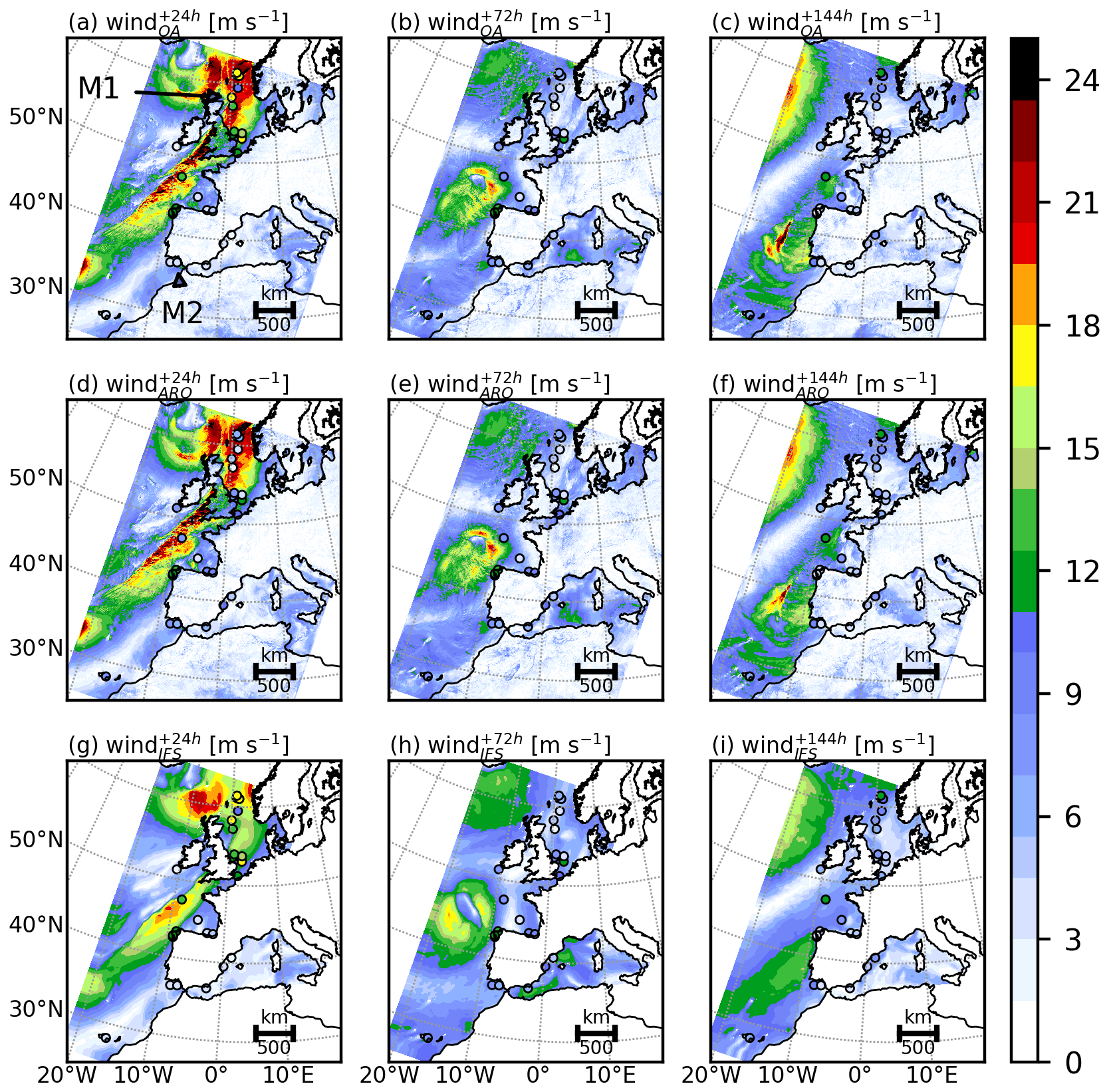
Figure 11Instantaneous 10 m ASL wind speed (m s−1) simulated by OA (a, b, c), ARO (d, e, f) and IFS seen by OCE-ifs (g, h, i), for forecast ranges of (a, d, g) +24 h (13 October 2018, 00:00 UTC), (b, e, h) +72 h (15 October 2018, 00:00 UTC) and (c, f, i) +144 h (18 October 2018, 00:00 UTC). The colour circles represent the wind speed measured by mooring buoys at that time; M1 and M2 labels in (a) indicate the location of the two mooring buoys used in Fig. 12.
Despite these overall spatial differences, the effect of the OA coupling does not significantly change the temporal evolution of the 10 m wind speed forecasts in comparison to OCE-aro-forced simulation and to mooring data (Fig. 12; 13). Note that the 10 m wind speed simulated by OCE-ifs has better scores than OA and ARO simulations at the mooring locations (Fig. 12), which can be explained by the wind overestimation in OA and ARO (as seen for M1 and M2 examples). Regarding the M1 moored buoy (58.3∘ N–0.1∘ E, northeast of the coasts of Scotland), however, OA reproduces the first wind peak in the afternoon of 12 October quite well but simulates a too strong and too early second peak on 13 October (Fig. 12a). Moderate wind (13 m s−1) is also simulated in the southwestern Mediterranean. The wind time series at M2 (36.4912∘ N, 6.9611∘ W, in the Gulf of Cadix, west of Gibraltar Strait) in Fig. 12b shows the good agreement of the OA simulation in this area. This can also be seen in the latest days in Fig. 12a, b.
The Taylor diagram in Fig. 12c summarizes the OA skill scores for the 7 d period, when compared to all in situ wind observations together, and to M1 and M2 separately. The mean bias is 1.3 m s−1, the standard deviation is 4.1 m s−1 and the correlation is 0.36 on average. This bias on AROME wind speed was already identified in Rainaud et al. (2016) and Léger et al. (2016), in particular for the strong wind situation and when comparing to coastal observing platforms. Further investigation would be needed to understand the origin of such a systematic bias, looking into both the AROME physics and the method to diagnose the wind at 10 m but is out of the scope of this paper.

Figure 12Temporal evolution of 10 m wind speed observed and simulated at the location of two moorings M1 (a) and M2 (b) (see Fig. 11a for locations). (c) Taylor diagrams made for the whole dataset of 44 selected moorings are shown as circles. Moorings M1 and M2 only are shown as squares and triangles respectively. The external colour indicates the experiment: blue for OA, purple for ARO (OCE-aro) and orange for IFS (OCE-ifs).
4.2.2 Rainfall
The temporal evolution of rainfall simulated by OA, ARO and OCE-ifs simulations is presented in Fig. 13e, f, g, h. The intensity of rainfall differs between the three simulations, but the chronology remains the same, except for the Mediterranean where there is more rainfall in IFS (OCE-ifs) than in AROME (ARO and OA). Hourly rainfall amounts exceed 10 mm in some places and are related to the passage of the various storms.
In the OA coupled simulation, the accumulated precipitation during the 7 simulated days is shown in Fig. 14a. Since we do not have the precipitation on land in the IFS data used to force NEMO, we cannot compare with the OCE-ifs simulation. The rain is heterogeneously distributed over the domain. In the Bay of Biscay, it follows the trajectory of Callum, with rainfall reaching 200 mm in the first 2 simulated days (Fig. 14c). In the Aude department (Fig. 14e), where the heavy precipitating event described in Sect. 3.1 occurred, the simulated accumulated precipitation reaches 300 mm in 1 d as observed but is located about 100 km to the east of the observed one. This location corresponds to the Massif Central relief (also known as the Cévennes), suggesting that the rapid and moist marine low-level flow is well reproduced, but with a slightly different orientation than observed and thus with a dominant triggering factor related to orographic uplift (whereas it was in fact related to convergence between the southeasterly flow with a cold front; Caumont et al., 2021). However, it is important to note that the Mediterranean HPE corresponds to forecast ranges between +66 and +90 h for AROME, i.e. quite far from the standard AROME forecast operational ranges. Despite the fact that observed and simulated intense precipitation amounts are not located exactly at the same place, the heavy precipitation signature with large values of rainfall amounts in only a few hours in the OA forecast appears very valuable in the context of very early warning of such severe events. We also highlight here the impact of the OA coupling on the rainfall amounts during the 7 d, as shown in Fig. 14b. The mean accumulated precipitation over the whole domain differs between the coupled and forced simulations by less than 0.5 %. However, total rainfall amounts can vary locally by more than 100 %, especially north of the Balearic Islands (40∘ N, 5∘ E) or close to Sicily (38∘ N, 15∘ E). Concerning the heavy precipitation that took place in Wales (Fig. 2), the differences between the OA and ARO simulations in total rainfall amounts during the first 48 h presented in Fig. 14d are quite small. The maximum differences reach about 20 mm and represent locally up to only 10 % of the 48 h cumulated rainfall amount. These differences are related to small displacements of the rain bands, linked to changes in the wind maxima localization discussed in the previous section (Fig. 11d). The effect of coupling is clearly visible for the Mediterranean heavy-precipitation event (see observed case in Fig. 2). Figure 14f shows that the 24 h rainfall amounts forecast in the OA simulation diverge from the ARO simulation. The precipitation areas are shifted in the OA simulation, which can be explained by the differences in low-level wind convergence position, which is a key triggering factor for mesoscale convective systems that generate heavy precipitation. This high sensitivity of wind convergence to sea surface structures and their evolution over the northwestern part of the Mediterranean Sea were already highlighted in previous studies (e.g. Rainaud et al., 2017; Meroni et al., 2018) and are there confirmed.
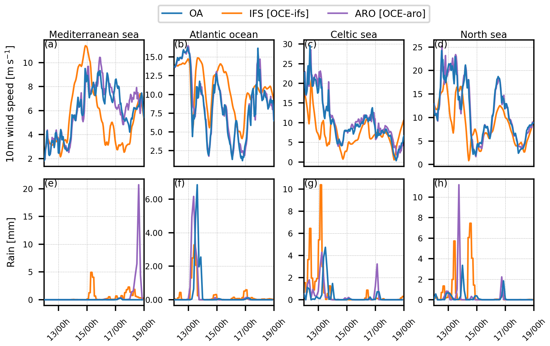
Figure 13Temporal evolution of simulated 10 m wind speed (m s−1; a, b, c, d) and rainfall (mm h−1 ; e, f, g, h) extracted in the four areas presented in Fig. 3d.

Figure 14Accumulated precipitation (mm) simulated by the coupled (OA) simulation (left column) and differences with the ARO-forced simulation (right column): (a, b) total amounts over the 7 d period, 24 h accumulated amounts (c, d) over the British Islands between 12 October, 00:00 UTC and 13 October, 00:00 UTC (+00 to +24 h forecast ranges) and (e, f) over the western Mediterranean area between 14 October, 18:00 UTC and 15 October, 18:00 UTC (between +66 and +90 h forecast ranges).
A new forecast-oriented high-resolution ocean–atmosphere coupled system using state-of-the-art AROME (cy43) and NEMO (3.6) models has been described in this paper. A new domain over western Europe, including the two domains used for high-resolution atmospheric and oceanic forecasts at Météo-France and Mercator Ocean International (MOI) respectively, has been designed. This coupled system was evaluated through 7 d simulations performed around an October 2018 study case. This case was chosen because during these 7 d, three storms and two intensive-rain periods occur over the simulated domain, which makes it a good candidate to study ocean–atmosphere coupling impacts, as air–sea interactions are exacerbated by such extreme conditions.
This new coupled system successfully simulates the different storms and their associated strong wind and surface turbulent fluxes. The maximum precipitation values of the two extreme rainfall events are also well simulated. Oceanic response associated with these extreme conditions shows significant vertical oceanic mixing along the storms' tracks. This mixing is responsible for an intense sea surface cooling of more than 1.5 ∘C in some places. Comparisons with observations (satellites and drifting buoys) show that this cooling is well localized even if too intense, notably in the Celtic Sea. This coupled system also successfully simulates the oceanic tides with their associated sea surface height and current variations. For this latter parameter notably, additional investigations will be needed to further explore the role of the current-feedback implementation in the AROME–NEMO coupled system.
To investigate the effect of OA coupling in the atmospheric and oceanic forecast, three additional simulations have been performed in a forced mode. Two simulations close to the current operational forecast systems operated at Météo-France and MOI respectively were run, and a third simulation with NEMO was set to understand the source of the main differences for ocean forecast. Indeed, compared to the closest simulation of the current operational system operated at MOI, the OA coupled system has two main differences: it uses a different atmospheric model (AROME versus IFS) with higher horizontal resolution (2.5 km compared to 9 km) and explicitly represents the ocean–atmosphere feedback. The different simulations show that the effect of changing the atmospheric model (and in particular its associated horizontal resolution) has a greater effect on the ocean forecast than taking into account the interactive air–sea feedback. The combined effect of both is visible on the surface fields, SST, SSS and currents but also on the structure of the oceanic mixed layer. It is explained by a stronger wind in the atmospheric forcing with AROME at 2.5 km horizontal resolution (+20 % in some places), which leads to stronger surface fluxes, and thus to a stronger oceanic response. Sea surface cooling can be higher than 6 ∘C in some places for our study case, it can affect the entire oceanic mixed layer and it is exacerbated where storms are located. The effect of ocean–atmosphere coupling on atmospheric forecast has been examined through comparison of simulated 10 m wind speed and accumulated precipitations with the forced simulation, in which SST is kept constant. Modifications due to coupling appear from the first simulated hours and increase over simulated time. The SST evolution in the OA simulation leads to changes in the location of the oceanic frontal structures notably, which induce changes in the wind convergence and thus in the location of the atmospheric convection areas and heavy rainfall. The coupling impact on the simulated wind and precipitation can vary up to 100 % in some places.
In summary, the coupled system slightly changes the atmospheric forecast on average even if strong differences are found locally for 10 m wind speed and rainfall amounts and significantly improves the sea surface temperature forecast (with a bias reduction of 30 %), when compared with the equivalent uncoupled forecast systems of Météo-France and MOI respectively and with the observations available over the simulation period and in our study area.
This work concretes our common first stage towards high-resolution ocean–atmosphere coupling for both oceanic and atmospheric forecasts. Thanks to our joint work for its update, with the development and application to a new region, the AROME–NEMO coupled system now permits further apprehension of operational regional ocean–atmosphere coupling in both institutes, Météo-France and Mercator Ocean International. It shows the affordability of such a numerical prediction system regarding the computation costs (see Appendix A) that can be shared and especially through the development of common tools.
Obviously, future challenges still remain for an operational implementation of such a high-resolution coupled system, in particular the insertion of a coupled data assimilation scheme and the issue of the data availability for both components, and coordinated code management with objectives of continuously improving the computing efficiency. Further investigations are also necessary to properly evaluate this new coupled system with respect to the current forecast systems. This must be done by enlarging the number of sensitivity case studies first, and then with a pre-operational set-up that will require consideration of the full forecast chains, from initialization with or without cycling (i.e. using or not using a previous coupled forecast) or assimilation, boundary condition extraction, forecast run, and downstream productions. At that stage only the qualification of the coupling system performances could be done, with the routine scores used to evaluate the actual operating systems, i.e. the dedicated NWP skill scores for AROME (Amodei et al., 2015) and the ocean validation results (described for IBI in Sotillo et al., 2021), as a careful quantification of the costs–benefits ratio of coupling.
All the developments are performed using a Vortex/Olive Python-based framework, used to run AROME operational simulations at Météo-France. This coupling system runs on the new Météo-France supercomputer Belenos (https://www.top500.org/system/179853/, last access: 7 April 2022). In total, this supercomputer has 294 912 cores on 2307 nodes and a peak performance of approximately 10.5 PFlop s−1. Each node has a random access memory (RAM) of 256 GB minimum.
Table A1 summarizes the computational cost of the different simulations presented in this article (Table 2).
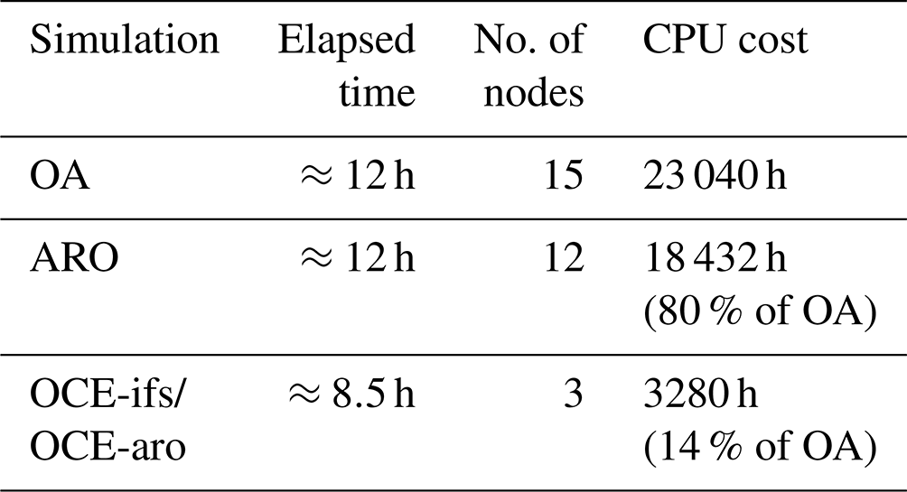
The coupled simulation runs on 15 nodes and 424 cores corresponding to 12 nodes and 384 cores for AROME, 2 nodes and 32 cores for NEMO, and 1 node and 8 cores for XIOS. Simulated time is roughly 12 h for AROME (ARO) and AROME–NEMO (OA) simulations, indicating that the effect of the OASIS coupler is negligible for this coupled system. The OA simulation CPU cost does not exactly correspond to the sum of the executions of AROME and NEMO/XIOS, as NEMO runs faster than AROME and therefore spends time waiting for it. It is indeed superior to the 18 432 CPU hours for one AROME forced (ARO) simulation plus the CPU cost of the oceanic model and the XIOS server for coupled AROME–NEMO (OA) simulation and finally corresponds to a 20 % total additional CPU cost (23 040 CPU hours). Note that simulated time of NEMO simulations alone (OCE-aro and OCE-ifs simulations) is roughly equal to 8.5 h (with 2 nodes and 32 cores for NEMO and 1 node and 8 cores for XIOS), corresponding to CPU cost of approximately 3280 CPU hours (14.2 % of the CPU cost of the OA coupled system). For the purpose of this comparison, we used the same number of nodes for NEMO simulations alone (OCE-aro and OCE-ifs simulations) as the one used in AROME–NEMO simulations, but it can be optimized, for example, by increasing the number of used cores by node.
Table A1Elapsed time and computational cost of the different 7 d simulations. One node contains 128 cores, and CPU cost is equal to elapsed time multiplied by the number of nodes multiplied by 128 (the number of cores multiplied by nodes) whatever the true number of nodes effectively used.
NEMO is available at https://www.nemo-ocean.eu/ (Madec et al., 2017; NEMO Community Ocean Model, 2022) after a user registration on the NEMO website. The version used is NEMO_v3.6.
OASIS3-MCT was used in version OASIS3-MCT_4.0. It can be downloaded at https://oasis.cerfacs.fr/en/ (Valcke, 2013; Craig et al., 2017; The Oasis Coupler, 2022). The public may copy, distribute, use, prepare derivative works and publicly display OASIS3-MCT under the terms of the Lesser GNU General Public License (LGPL) as published by the Free Software Foundation, provided that this notice and any statement of authorship are reproduced on all copies.
SURFEX open-source version (Open-SURFEX) including the interface with OASIS from v8_0 is available at http://www.umr-cnrm.fr/surfex/ (Masson et al., 2013; SURFEX, 2022) using a CECILL-C Licence (a French equivalent of the L-GPL licence; http://www.cecill.info/licences/Licence_CeCILL-C_V1-en.txt, CeCILL-C Free Software License Agreement, 2022), but with the exception of the Gaussian grid projection, the LFI and FA I/O formats, and the dr HOOK tool.
Although the operational AROME code cannot be obtained, the modified sources for cy43 are available on demand to the authors for the partners of the ACCORD consortium and are included in the new Météo-France official release based on cycle 48 (cy48t1).
Outputs from all simulations discussed here are available upon request to the authors.
The moored and drifting buoy data were collected and made freely available by the Coriolis project and programmes that contribute to it (http://www.coriolis.eu.org, Coriolis Operational Oceanography, 2022). The L3S SST satellite data were provided by GHRSST and the CMEMS Regional Data Assembly Centre.
FES2014 was produced by Noveltis, Legos and CLS and distributed by Aviso+, with support from CNES (https://www.aviso.altimetry.fr/, AVISO+ Satellite Altimetry Data, 2000; Carrere et al., 2015).
All authors (JP, JB, CLB, GS, GF and GG) contributed to the conceptualization and methodology of the study as well as drafting, reviewing and editing of the article. GF finalized the Vortex/Olive-Swapp experimental configuration for coupled simulations and extracted the IFS forecast files. The configurations NEMO-eNEATL36 and AROME-Mercator were developed by JP and JB, who also ran the coupled and uncoupled simulations. JP, JB, CLB, GS and GG carried out the analysis of the results.
The contact author has declared that neither they nor their co-authors have any competing interests.
Publisher’s note: Copernicus Publications remains neutral with regard to jurisdictional claims in published maps and institutional affiliations.
The authors thank Sylvie Malardel, Soline Bielli (LACy), Sébastien Riette (CNRM) and the SWAPP system team (Météo-France), who helped us in the implementation of the coupled experiment design in the Vortex/Olive-Swapp environment.
This work was funded by Mercator Ocean International.
This paper was edited by Piero Lionello and reviewed by two anonymous referees.
Amodei, M., Sanchez, I., and Stein, J.: Verification of the French operational high-resolution model AROME with the regional Brier probability score, Meteorol. Appl., 22, 731–745, https://doi.org/10.1002/met.1510, 2015. a
Arnold, A. K., Lewis, H. W., Hyder, P., Siddorn, J., and O'Dea, E.: The Sensitivity of British Weather to Ocean Tides, Geophys. Res. Lett., 48, e2020GL090732, https://doi.org/10.1029/2020GL090732, 2021. a
AVISO+ Satellite Altimetry Data: https://www.aviso.altimetry.fr/en/home.html, last access: 7 April 2022. a
Bao, J.-W., Wilczak, J. M., Choi, J.-K., and Kantha, L. H.: Numerical Simulations of Air-Sea Interaction under High Wind Conditions Using a Coupled Model: A Study of Hurricane Development, Mon. Weather Rev., 128, 2190–2210, https://doi.org/10.1175/1520-0493(2000)128<2190:NSOASI>2.0.CO;2, 2000. a
Barnier, B., Madec, G., Penduff, T., Molines, J.-M., Treguier, A.-M., Le Sommer, J., Beckmann, A., Biastoch, A., Böning, C., Dengg, J., Derval, C., Durand, E., Gulev, S., Remy, E., Talandier, C., Theetten, S., Maltrud, M., McClean, J., and De Cuevas, B.: Impact of partial steps and momentum advection schemes in a global ocean circulation model at eddy-permitting resolution, Ocean Dynam., 56, 543–567, https://doi.org/10.1007/s10236-006-0082-1, 2006. a
Bastin, S., Drobinski, P., Guénard, V., Caccia, J.-L., Campistron, B., Dabas, A. M., Delville, P., Reitebuch, O., and Werner, C.: On the Interaction between Sea Breeze and Summer Mistral at the Exit of the Rhône Valley, Mon. Weather Rev., 134, 1647–1668, https://doi.org/10.1175/MWR3116.1, 2006. a
Bender, M. A. and Ginis, I.: Real-Case Simulations of Hurricane–Ocean Interaction Using A High-Resolution Coupled Model: Effects on Hurricane Intensity, Mon. Weather Rev., 128, 917–946, https://doi.org/10.1175/1520-0493(2000)128<0917:RCSOHO>2.0.CO;2, 2000. a
Bergeron, J.-P.: Contrasting years in the Gironde estuary (Bay of Biscay, NE Atlantic) springtime outflow and consequences for zooplankton pyruvate kinase activity and the nutritional condition of anchovy larvae: an early view, ICES J. Mar. Sci., 61, 928–932, https://doi.org/10.1016/j.icesjms.2004.06.019, 2004. a
Blayo, E. and Debreu, L.: Revisiting open boundary conditions from the point of view of characteristic variables, Ocean Model., 9, 231–252, https://doi.org/10.1016/j.ocemod.2004.07.001, 2005. a
Bouin, M.-N. and Lebeaupin Brossier, C.: Surface processes in the 7 November 2014 medicane from air–sea coupled high-resolution numerical modelling, Atmos. Chem. Phys., 20, 6861–6881, https://doi.org/10.5194/acp-20-6861-2020, 2020a. a
Bouin, M.-N. and Lebeaupin Brossier, C.: Impact of a medicane on the oceanic surface layer from a coupled, kilometre-scale simulation, Ocean Sci., 16, 1125–1142, https://doi.org/10.5194/os-16-1125-2020, 2020b. a
Brassington, G., Martin, M., Tolman, H., Akella, S., Balmeseda, M., Chambers, C., Chassignet, E., Cummings, J., Drillet, Y., Jansen, P., Laloyaux, P., Lea, D., Mehra, A., Mirouze, I., Ritchie, H., Samson, G., Sandery, P., Smith, G., Suarez, M., and Todling, R.: Progress and challenges in short- to medium-range coupled prediction, J. Oper. Oceanogr., 8, s239–s258, https://doi.org/10.1080/1755876X.2015.1049875, 2015. a
Brenon, I. and Le Hir, P.: Modelling the Turbidity Maximum in the Seine Estuary (France): Identification of Formation Processes, Estuar. Coast. Shelf S., 49, 525–544, https://doi.org/10.1006/ecss.1999.0514, 1999. a
Brousseau, P., Seity, Y., Ricard, D., and Léger, J.: Improvement of the forecast of convective activity from the AROME-France system, Q. J. Roy. Meteor. Soc., 142, 2231–2243, https://doi.org/10.1002/qj.2822, 2016. a
Carniel, S., Benetazzo, A., Bonaldo, D., Falcieri, F. M., Miglietta, M. M., Ricchi, A., and Sclavo, M.: Scratching beneath the surface while coupling atmosphere, ocean and waves: Analysis of a dense water formation event, Ocean Model., 101, 101–112, https://doi.org/10.1016/j.ocemod.2016.03.007, 2016. a
Carrere, L., Lyard, F., Cancet, M., and Guillot, A.: FES 2014, a new tidal model on the global ocean with enhanced accuracy in shallow seas and in the Arctic region, in: EGU General Assembly Conference Abstracts, Vienna, Austria, 12–17 April 2015, 5481 pp., EGU General Assembly Conference Abstracts, 2015. a, b
Carret, A., Birol, F., Estournel, C., Zakardjian, B., and Testor, P.: Synergy between in situ and altimetry data to observe and study Northern Current variations (NW Mediterranean Sea), Ocean Sci., 15, 269–290, https://doi.org/10.5194/os-15-269-2019, 2019. a
Caumont, O., Mandement, M., Bouttier, F., Eeckman, J., Lebeaupin Brossier, C., Lovat, A., Nuissier, O., and Laurantin, O.: The heavy precipitation event of 14–15 October 2018 in the Aude catchment: a meteorological study based on operational numerical weather prediction systems and standard and personal observations, Nat. Hazards Earth Syst. Sci., 21, 1135–1157, https://doi.org/10.5194/nhess-21-1135-2021, 2021. a, b
CeCILL-C Free Software License Agreement: https://www.cecill.info/licences/Licence_CeCILL-C_V1-en.txt, last access: 7 April 2022. a
Charnock, H.: Wind stress on a water surface, Q. J. Roy. Meteor. Soc., 81, 639–640, https://doi.org/10.1002/qj.49708135027, 1955. a
Chen, S., Campbell, T. J., Jin, H., Gabersek, S., Hodur, R. M., and Martin, P.: Effect of Two-Way Air–Sea Coupling in High and Low Wind Speed Regimes, Mon. Weather Rev., 138, 3579–3602, https://doi.org/10.1175/2009MWR3119.1, 2010. a
Chevallier, C., Herbette, S., Marié, L., Le Borgne, P., Marsouin, A., Péré, S., Levier, B., and Reason, C.: Observations of the Ushant front displacements with MSG/SEVIRI derived sea surface temperature data, in: Remote sensing of ocean colour, temperature and salinity, Remote Sens. Environ., 146, 3–10, https://doi.org/10.1016/j.rse.2013.07.038, 2014. a
Colella, S., Böhm, E., Cesarini, C., Garnesson, P., Netting, J., and Calton, B.: Product User Manual for All Ocean Colour Products (CMEMS-OC-PUM-009-ALL), Tech. rep., Copernicus Marine Environment Monitoring Service, https://catalogue.marine.copernicus.eu/documents/PUM/CMEMS-OC-PUM-009-ALL.pdf (last access: 7 April 2022), 2020. a
Coriolis Operational Oceanography: Measurements for Ocean Understanding, The Coriolis Project, https://www.coriolis.eu.org/, last access: 7 April 2022. a
Courtier, P., Freydier, C., Geleyn, J.-F., Rabier, F., and Rochas, M.: The ARPEGE project at Météo-France, in: ECMWF workshop on numerical methods in atmospheric modeling, ECMW, Reading, UK, 2, 193–231, 1991. a
Craig, A., Valcke, S., and Coquart, L.: Development and performance of a new version of the OASIS coupler, OASIS3-MCT_3.0, Geosci. Model Dev., 10, 3297–3308, https://doi.org/10.5194/gmd-10-3297-2017, 2017. a, b
Cuxart, J., Bougeault, P., and Redelsperger, J.-L.: A turbulence scheme allowing for mesoscale and large-eddy simulations, Q. J. Roy. Meteor. Soc., 126, 1–30, https://doi.org/10.1002/qj.49712656202, 2000. a
Darmaraki, S., Somot, S., Sevault, F., Nabat, P., Cabos Narvaez, W. D., Cavicchia, L., Djurdjevic, V. m., Li, L., Sannino, G., and Sein, D. V.: Future evolution of Marine Heatwaves in the Mediterranean Sea, Clim. Dynam., 53, 1371–1392, https://doi.org/10.1007/s00382-019-04661-z, 2019. a
De Bono, A., Peduzzi, P., Kluser, S., and Giuliani, G.: Impacts of Summer 2003 Heat Wave in Europe, 4, https://archive-ouverte.unige.ch/unige:32255 (last access: 7 April 2022), 2004. a
D'Ortenzio, F., Iudicone, D., de Boyer Montegut, C., Testor, P., Antoine, D., Marullo, S., Santoleri, R., and Madec, G.: Seasonal variability of the mixed layer depth in the mediterranean sea as derived from in situ profiles, Geophys. Res. Lett., 32, L12605, https://doi.org/10.1029/2005GL022463, 2005. a
Ducrocq, V., Davolio, S., Ferretti, R., Flamant, C., Homar Santaner, V., Kalthoff, N., Richard, E., and Wernli, H.: Advances in understanding and forecasting of heavy precipitation in Mediterranean through the HyMeX SOP1 field campaign, Q. J. Roy. Meteor. Soc., 142, 1–6, https://doi.org/10.1002/qj.2856, 2016. a
Echevin, V., Crepon, M., and Mortier, L.: Interaction of a Coastal Current with a Gulf: Application to the Shelf Circulation of the Gulf of Lions in the Mediterranean Sea, J. Phys. Oceanogr., 33, 188–206, https://doi.org/10.1175/1520-0485(2003)033<0188:IOACCW>2.0.CO;2, 2003. a
ECMWF: IFS Documentation CY47R1, https://www.ecmwf.int/en/publications/ifs-documentation (last access: 7 April 2022), 2020. a, b
Estournel, C., Broche, P., Marsaleix, P., Devenon, J.-L., Auclair, F., and Vehil, R.: The Rhone River Plume in Unsteady Conditions: Numerical and Experimental Results, Estuar. Coast. Shelf S., 53, 25–38, https://doi.org/10.1006/ecss.2000.0685, 2001. a
Eyring, V., Bony, S., Meehl, G. A., Senior, C. A., Stevens, B., Stouffer, R. J., and Taylor, K. E.: Overview of the Coupled Model Intercomparison Project Phase 6 (CMIP6) experimental design and organization, Geosci. Model Dev., 9, 1937–1958, https://doi.org/10.5194/gmd-9-1937-2016, 2016. a
Fairall, C. W., Bradley, E. F., Hare, J. E., Grachev, A. A., and Edson, J. B.: Bulk Parameterization of Air-Sea Fluxes: Updates and Verification for the COARE Algorithm, J. Climate, 16, 571–591, https://doi.org/10.1175/1520-0442(2003)016<0571:BPOASF>2.0.CO;2, 2003. a, b
Fouquart, Y. and Bonnel, B.: Computations of Solar Heating of the Earth’s Atmosphere: A New Parameterization, Beitrage zur Physik der Atmosphare, 53, 35–62, 1980. a
Fujiwhara, S.: The natural tendency towards symmetry of motion and its application as a principle in meteorology, Q. J. Roy. Meteor. Soc., 47, 287–293, 1921. a
García, M. J. L., Millot, C., Font, J., and García-Ladona, E.: Surface circulation variability in the Balearic Basin, J. Geophys. Res.-Oceans, 99, 3285–3296, https://doi.org/10.1029/93JC02114, 1994. a
Grifoll, M., Navarro, J., Pallares, E., Ràfols, L., Espino, M., and Palomares, A.: Ocean–atmosphere–wave characterisation of a wind jet (Ebro shelf, NW Mediterranean Sea), Nonlinear Proc. Geoph., 23, 143–158, https://doi.org/10.5194/npg-23-143-2016, 2016. a
Gutknecht, E., Reffray, G., Mignot, A., Dabrowski, T., and Sotillo, M. G.: Modelling the marine ecosystem of Iberia–Biscay–Ireland (IBI) European waters for CMEMS operational applications, Ocean Sci., 15, 1489–1516, https://doi.org/10.5194/os-15-1489-2019, 2019. a
Hewitt, H. T., Roberts, M., Mathiot, P., Biastoch, A., Blockley, E., Chassignet, E. P., Fox-Kemper, B., Hyder, P., Marshall, D. P., Popova, E., Treguier, A.-M., Zanna, L., Yool, A., Yu, Y., Beadling, R., Bell, M., Kuhlbrodt, T., Arsouze, T., Bellucci, A., Castruccio, F., Gan, B., Putrasahan, D., Roberts, C. D., Van Roekel, L., and Zhang, Q.: Resolving and Parameterising the Ocean Mesoscale in Earth System Models, Current Climate Change Reports, 6, 137–152, https://doi.org/10.1007/s40641-020-00164-w, 2020. a
Intergovernmental Panel on Climate Change: Climate Change 2013 – The Physical Science Basis: Working Group I Contribution to the Fifth Assessment Report of the Intergovernmental Panel on Climate Change, Cambridge University Press, Cambridge, https://doi.org/10.1017/CBO9781107415324, 2014. a
Jullien, S., Marchesiello, P., Menkes, C. E., Lefèvre, J., Jourdain, N. C., Samson, G., and Lengaigne, M.: Ocean feedback to tropical cyclones: climatology and processes, Clim. Dynam., 43, 2831–2854, https://doi.org/10.1007/s00382-014-2096-6, 2014. a
Jullien, S., Masson, S., Oerder, V., Samson, G., Colas, F., and Renault, L.: Impact of Ocean-Atmosphere Current Feedback on Ocean Mesoscale Activity: Regional Variations and Sensitivity to Model Resolution, J. Climate, 33, 2585–2602, https://doi.org/10.1175/JCLI-D-19-0484.1, 2020. a
Kain, J. S. and Fritsch, J. M.: A One-Dimensional Entraining/Detraining Plume Model and Its Application in Convective Parameterization, Journal of Atmospheric Sciences, 47, 2784–2802, https://doi.org/10.1175/1520-0469(1990)047<2784:AODEPM>2.0.CO;2, 1990. a
Kendon, M., McCarthy, M., Jevrejeva, S., Matthews, A., and Legg, T.: State of the UK climate 2018, Int. J. Climatol., 39, 1–55, https://doi.org/10.1002/joc.6213, 2019. a, b
Le Boyer, A., Charria, G., Le Cann, B., Lazure, P., and Marié, L.: Circulation on the shelf and the upper slope of the Bay of Biscay, Cont. Shelf Res., 55, 97–107, https://doi.org/10.1016/j.csr.2013.01.006, 2013. a
Lebeaupin Brossier, C., Léger, F., Giordani, H., Beuvier, J., Bouin, M., Ducrocq, V., and Fourrié, N.: Dense water formation in the north‐western Mediterranean area during HyMeX‐SOP2 in 1/36∘ ocean simulations: Ocean‐atmosphere coupling impact, J. Geophys. Res.-Oceans, 122, 5749–5773, https://doi.org/10.1002/2016JC012526, 2017. a, b, c, d
Leclair, M. and Madec, G.: A conservative leapfrog time stepping method, Ocean Model., 30, 88–94, https://doi.org/10.1016/j.ocemod.2009.06.006, 2009. a
Lellouche, J.-M., Greiner, E., Le Galloudec, O., Garric, G., Regnier, C., Drevillon, M., Benkiran, M., Testut, C.-E., Bourdalle-Badie, R., Gasparin, F., Hernandez, O., Levier, B., Drillet, Y., Remy, E., and Le Traon, P.-Y.: Recent updates to the Copernicus Marine Service global ocean monitoring and forecasting real-time 1∕12∘ high-resolution system, Ocean Sci., 14, 1093–1126, https://doi.org/10.5194/os-14-1093-2018, 2018. a
Lewis, H. W., Castillo Sanchez, J. M., Arnold, A., Fallmann, J., Saulter, A., Graham, J., Bush, M., Siddorn, J., Palmer, T., Lock, A., Edwards, J., Bricheno, L., Martínez-de la Torre, A., and Clark, J.: The UKC3 regional coupled environmental prediction system, Geosci. Model Dev., 12, 2357–2400, https://doi.org/10.5194/gmd-12-2357-2019, 2019. a
Liberato, M. L. R., Pinto, J. G., Trigo, R. M., Ludwig, P., Ordóñez, P., Yuen, D., and Trigo, I. F.: Explosive development of winter storm Xynthia over the subtropical North Atlantic Ocean, Nat. Hazards Earth Syst. Sci., 13, 2239–2251, https://doi.org/10.5194/nhess-13-2239-2013, 2013. a
Ličer, M., Smerkol, P., Fettich, A., Ravdas, M., Papapostolou, A., Mantziafou, A., Strajnar, B., Cedilnik, J., Jeromel, M., Jerman, J., Petan, S., Malačič, V., and Sofianos, S.: Modeling the ocean and atmosphere during an extreme bora event in northern Adriatic using one-way and two-way atmosphere–ocean coupling, Ocean Sci., 12, 71–86, https://doi.org/10.5194/os-12-71-2016, 2016. a
Léger, F., Lebeaupin Brossier, C., Giordani, H., Arsouze, T., Beuvier, J., Bouin, M.-N., Bresson, E., Ducrocq, V., Fourrié, N., and Nuret, M.: Dense water formation in the north-western Mediterranean area during HyMeX-SOP2 in 1/36∘ ocean simulations: Sensitivity to initial conditions, J. Geophys. Res.-Oceans, 121, 5549–5569, https://doi.org/10.1002/2015JC011542, 2016. a
Ma, F., Yuan, X., Jiao, Y., and Ji, P.: Unprecedented Europe Heat in June–July 2019: Risk in the Historical and Future Context, Geophys. Res. Lett., 47, e2020GL087809, https://doi.org/10.1029/2020GL087809, 2020. a
Madec, G., Bourdallé-Badie, R., Pierre-Antoine Bouttier, Bricaud, C., Bruciaferri, D., Calvert, D., Chanut, J., Clementi, E., Coward, A., Delrosso, D., Ethé, C., Flavoni, S., Graham, T., Harle, J., Iovino, D., Lea, D., Lévy, C., Lovato, T., Martin, N., Masson, S., Mocavero, S., Paul, J., Rousset, C., Storkey, D., Storto, A., and Vancoppenolle, M.: NEMO ocean engine, Zenodo [software], https://doi.org/10.5281/ZENODO.1472492, 2017. a, b
Mandement, M. and Caumont, O.: A numerical study to investigate the roles of former Hurricane Leslie, orography and evaporative cooling in the 2018 Aude heavy-precipitation event, Weather Clim. Dynam., 2, 795–818, https://doi.org/10.5194/wcd-2-795-2021, 2021. a
Maraldi, C., Chanut, J., Levier, B., Ayoub, N., De Mey, P., Reffray, G., Lyard, F., Cailleau, S., Drévillon, M., Fanjul, E. A., Sotillo, M. G., Marsaleix, P., and the Mercator Research and Development Team: NEMO on the shelf: assessment of the Iberia–Biscay–Ireland configuration, Ocean Sci., 9, 745–771, https://doi.org/10.5194/os-9-745-2013, 2013. a
Masson, V.: A Physically-Based Scheme For The Urban Energy Budget In Atmospheric Models, Bound.-Lay. Meteorol., 94, 357–397, https://doi.org/10.1023/A:1002463829265, 2000. a
Masson, V., Le Moigne, P., Martin, E., Faroux, S., Alias, A., Alkama, R., Belamari, S., Barbu, A., Boone, A., Bouyssel, F., Brousseau, P., Brun, E., Calvet, J.-C., Carrer, D., Decharme, B., Delire, C., Donier, S., Essaouini, K., Gibelin, A.-L., Giordani, H., Habets, F., Jidane, M., Kerdraon, G., Kourzeneva, E., Lafaysse, M., Lafont, S., Lebeaupin Brossier, C., Lemonsu, A., Mahfouf, J.-F., Marguinaud, P., Mokhtari, M., Morin, S., Pigeon, G., Salgado, R., Seity, Y., Taillefer, F., Tanguy, G., Tulet, P., Vincendon, B., Vionnet, V., and Voldoire, A.: The SURFEXv7.2 land and ocean surface platform for coupled or offline simulation of earth surface variables and fluxes, Geosci. Model Dev., 6, 929–960, https://doi.org/10.5194/gmd-6-929-2013, 2013. a, b
Meehl, G. A.: Development of global coupled ocean-atmosphere general circulation models, Clim. Dynam., 5, 19–33, https://doi.org/10.1007/BF00195851, 1990. a
Meroni, A. N., Renault, L., Parodi, A., and Pasquero, C.: Role of the Oceanic Vertical Thermal Structure in the Modulation of Heavy Precipitations Over the Ligurian Sea, Pure App. Geophys., 175, 4111–4130, https://doi.org/10.1007/s00024-018-2002-y, 2018. a, b
Meurdesoif, Y.: XIOS, in: Second Workshop on Coupling Technologies for Earth System Models (CW2013), NCAR, Boulder, CO, USA, http://forge.ipsl.jussieu.fr/ioserver/raw-attachment/wiki/WikiStart/XIOS-BOULDER.pdf (last access: 7 April 2022), 2013. a
Miglietta, M. M. and Rotunno, R.: Development mechanisms for Mediterranean tropical-like cyclones (medicanes), Q. J. Roy. Meteor. Soc., 145, 1444–1460, https://doi.org/10.1002/qj.3503, 2019. a
Millot, C.: Mesoscale and seasonal variabilities of the circulation in the western Mediterranean, Dyn. Atmos. Oc., 15, 179–214, https://doi.org/10.1016/0377-0265(91)90020-G, 1991. a
Millot, C. and Taupier-Letage, I.: Circulation in the Mediterranean Sea, in: The Mediterranean Sea, edited by: Saliot, A., Springer Berlin Heidelberg, Berlin, Heidelberg, 29–66, https://doi.org/10.1007/b107143, 2005. a
Millot, C., Taupier-Letage, I., and Benzohra, M.: The Algerian eddies, Earth-Sci. Rev., 27, 203–219, https://doi.org/10.1016/0012-8252(90)90003-E, 1990. a
Mlawer, E. J., Taubman, S. J., Brown, P. D., Iacono, M. J., and Clough, S. A.: Radiative transfer for inhomogeneous atmospheres: RRTM, a validated correlated-k model for the longwave, J. Geophys. Res.-Atmos., 102, 16663–16682, https://doi.org/10.1029/97JD00237, 1997. a
Mogensen, K. S., Hewson, T., Keeley, S., and Magnusson, L.: Effects of ocean coupling on weather forecasts, ECMWF newsletter, 6–7, https://www.ecmwf.int/en/newsletter/156/news/effects-ocean-coupling-weather-forecasts (last access: 7 April 2022), 2018. a
NEMO Community Ocean Model: https://www.nemo-ocean.eu/, last access: 7 April 2022. a
Noilhan, J. and Planton, S.: A Simple Parameterization of Land Surface Processes for Meteorological Models, Mon. Weather Rev., 117, 536–549, https://doi.org/10.1175/1520-0493(1989)117<0536:ASPOLS>2.0.CO;2, 1989. a
Obermann, A., Bastin, S., Belamari, S., Conte, D., Gaertner, M. A., Li, L., and Ahrens, B.: Mistral and Tramontane wind speed and wind direction patterns in regional climate simulations, Clim. Dynam., 51, 1059–1076, https://doi.org/10.1007/s00382-016-3053-3, 2018. a
Orain, F., Roquet, H., and Saux Picart, E.: European Near Real Time Level 3S Sea Surface Temperature Product SST_EUR_L3S_NRT_OBSERVATIONS_010_009_a, Quality Information Document #1.6, Tech. rep., Copernicus Marine Environment Monitoring Service, 16 pp., https://catalogue.marine.copernicus.eu/documents/QUID/CMEMS-SST-QUID-010-009-a.pdf (last access: 7 April 2022), 2021. a
Pasch, R. J. and Roberts, D. P.: Hurricane Leslie, National Hurricane Center Tropical Cyclone Report, Tech. rep. AL132018, 18 pp., https://www.nhc.noaa.gov/data/tcr/AL132018_Leslie.pdf(last access: 7 April 2022), 2019. a
Pellerin, P., Ritchie, H., Saucier, F. J., Roy, F., Desjardins, S., Valin, M., and Lee, V.: Impact of a Two-Way Coupling between an Atmospheric and an Ocean-Ice Model over the Gulf of St. Lawrence, Mon. Weather Rev., 132, 1379–1398, https://doi.org/10.1175/1520-0493(2004)132<1379:IOATCB>2.0.CO;2, 2004. a
Pianezze, J., Barthe, C., Bielli, S., Tulet, P., Jullien, S., Cambon, G., Bousquet, O., Claeys, M., and Cordier, E.: A New Coupled Ocean-Waves-Atmosphere Model Designed for Tropical Storm Studies: Example of Tropical Cyclone Bejisa (2013–2014) in the South-West Indian Ocean, J. Adv. Model. Earth Sy., 10, 801–825, https://doi.org/10.1002/2017MS001177, 2018. a
Pinty, J.-P. and Jabouille, P.: A mixed-phase cloud parameterization for use in a mesoscale non-hydrostatic model: simulations of a squall line and of orographic precipitation, in: Proceedings of the AMS conference on cloud physics, Amer. Meteor. soc., Everett, WA, USA, 17–21 August 1998, 217–220, http://mesonh.aero.obs-mip.fr/mesonh/dir_publication/pinty_jabouille_ams_ccp1998.pdf, 1998. a
Pullen, J., Doyle, J. D., and Signell, R. P.: Two-way air-sea coupling: A study of the Adriatic, Mon. Wea. Rev., 135, 1465–1483, https://doi.org/10.1175/MWR3137.1, 2006. a
Pullen, J., Allard, R., Seo, H., Miller, A. J., Chen, S., Pezzi, L. P., Smith, T., Chu, P., Alves, J., and Caldeira, R.: Coupled ocean-atmosphere forecasting at short and medium time scales, J. Mar. Res., 75, 877–921, https://doi.org/10.1357/002224017823523991, 2017. a
Rainaud, R., Lebeaupin Brossier, C., Ducrocq, V., Giordani, H., Nuret, M., Fourrié, N., Bouin, M.-N., Taupier-Letage, I., and Legain, D.: Characterization of air–sea exchanges over the Western Mediterranean Sea during HyMeX SOP1 using the AROME–WMED model, Q. J. Roy. Meteor. Soc., 142, 173–187, https://doi.org/10.1002/qj.2480, 2016. a
Rainaud, R., Lebeaupin Brossier, C., Ducrocq, V., and Giordani, H.: High-resolution air-sea coupling impact on two heavy precipitation events in the Western Mediterranean: Air-Sea Coupling Impact on Two Mediterranean HPEs, Q. J. Roy. Meteor. Soc., 143, 2448–2462, https://doi.org/10.1002/qj.3098, 2017. a, b, c, d, e, f
Redelsperger, J.-L., Bouin, M.-N., Pianezze, J., Garnier, V., and Marié, L.: Impact of a sharp, small-scale SST front on the marine atmospheric boundary layer on the Iroise Sea: Analysis from a hectometric simulation, Q. J. Roy. Meteor. Soc., 145, 3692–3714, https://doi.org/10.1002/qj.3650, 2019. a
Renault, L., Lemarié, F., and Arsouze, T.: On the implementation and consequences of the oceanic currents feedback in ocean–atmosphere coupled models, Ocean Model., 141, 101423, https://doi.org/10.1016/j.ocemod.2019.101423, 2019a. a
Renault, L., Marchesiello, P., Masson, S., and McWilliams, J. C.: Remarkable Control of Western Boundary Currents by Eddy Killing , a Mechanical Air‐Sea Coupling Process, Geophys. Res. Lett., 46, 2743–2751, https://doi.org/10.1029/2018GL081211, 2019b. a
Sauvage, C., Lebeaupin Brossier, C., and Bouin, M.-N.: Towards kilometer-scale ocean–atmosphere–wave coupled forecast: a case study on a Mediterranean heavy precipitation event, Atmos. Chem. Phys., 21, 11857–11887, https://doi.org/10.5194/acp-21-11857-2021, 2021. a
Seity, Y., Brousseau, P., Malardel, S., Hello, G., Bénard, P., Bouttier, F., Lac, C., and Masson, V.: The AROME-France Convective-Scale Operational Model, Mon. Weather Rev., 139, 976–991, https://doi.org/10.1175/2010MWR3425.1, 2011. a
Shukla, J., Palmer, T. N., Hagedorn, R., Hoskins, B., Kinter, J., Marotzke, J., Miller, M., and Slingo, J.: Toward a New Generation of World Climate Research and Computing Facilities, B. Am. Meteorol. Soc., 91, 1407–1412, https://doi.org/10.1175/2010BAMS2900.1, 2010. a
Simpson, J. H., Bos, W. G., Schirmer, F., Souza, A. J., Rippeth, T. P., Jones, S. E., and Hydes, D.: Periodic stratification in the rhine ROFI in the north-sea, https://archimer.ifremer.fr/doc/00099/21050/ (last access: 7 April 2022), 1993. a
Small, R., Carniel, S., Campbell, T., Teixeira, J., and Allard, R.: The response of the Ligurian and Tyrrhenian Seas to a summer Mistral event: A coupled atmosphere–ocean approach, Ocean Model., 48, 30–44, https://doi.org/10.1016/j.ocemod.2012.02.003, 2012. a
Small, R. J., Campbell, T., Teixeira, J., Carniel, S., Smith, T. A., Dykes, J., Chen, S., and Allard, R.: Air-Sea Interaction in the Ligurian Sea: Assessment of a Coupled Ocean-Atmosphere Model Using In Situ Data from LASIE07, Mon. Weather Rev., 139, 1785–1808, https://doi.org/10.1175/2010MWR3431.1, 2011. a
Smith, R. K., Montgomery, M. T., and Van Sang, N.: Tropical cyclone spin-up revisited, Q. J. Roy. Meteor. Soc., 135, 1321–1335, https://doi.org/10.1002/qj.428, 2009. a
Sotillo, M. G., Cailleau, S., Lorente, P., Levier, B., Aznar, R., Reffray, G., Amo-Baladron, A., Chanut, J., Benkiran, M., and Alvarez-Fanjul, E.: The MyOcean IBI Ocean Forecast and Reanalysis Systems: operational products and roadmap to the future Copernicus Service, J. Oper. Oceanogr., 8, 63–79, https://doi.org/10.1080/1755876X.2015.1014663, 2015. a, b
Sotillo, M. G., Levier, B., Lorente, P., Guihou, K., Aznar, R., Amo, A., Aouf, L., and Ghantous, M.: Quality information document for Atlantic -Iberian Biscay Irish-Ocean Physics Analysis and Forecasting Product (CMEMS-IBI-QUID-005-001), Copernicus Marine Environment Monitoring Service, Tech. rep., 120 pp., https://catalogue.marine.copernicus.eu/documents/QUID/CMEMS-IBI-QUID-005-001.pdf, 2021. a, b, c, d
Stockdale, T. N., Anderson, D. L. T., Alves, J. O. S., and Balmaseda, M. A.: Global seasonal rainfall forecasts using a coupled ocean–atmosphere model, Nature, 392, 370–373, https://doi.org/10.1038/32861, 1998. a
SURFEX: https://www.umr-cnrm.fr/surfex/, last access: 7 April 2022. a
Szekely, T., Gourrion, J., Pouliquen, S., and Reverdin, G.: The CORA 5.2 dataset for global in situ temperature and salinity measurements: data description and validation, Ocean Sci., 15, 1601–1614, https://doi.org/10.5194/os-15-1601-2019, 2019. a
Taszarek, M., Allen, J., Púčik, T., Groenemeijer, P., Czernecki, B., Kolendowicz, L., Lagouvardos, K., Kotroni, V., and Schulz, W.: A Climatology of Thunderstorms across Europe from a Synthesis of Multiple Data Sources, J. Climate, 32, 1813–1837, https://doi.org/10.1175/JCLI-D-18-0372.1, 2019. a
Taylor, J. P., Edwards, J. M., Glew, M. D., Hignett, P., and Slingo, A.: Studies with a flexible new radiation code. II: Comparisons with aircraft short-wave observations, Q. J. Roy. Meteor. Soc., 122, 839–861, https://doi.org/10.1002/qj.49712253204, 1996. a
Testor, P., Bosse, A., Houpert, L., Margirier, F., Mortier, L., Legoff, H., Dausse, D., Labaste, M., Karstensen, J., Hayes, D., Olita, A., Ribotti, A., Schroeder, K., Chiggiato, J., Onken, R., Heslop, E., Mourre, B., D'ortenzio, F., Mayot, N., Lavigne, H., de Fommervault, O., Coppola, L., Prieur, L., Taillandier, V., Durrieu de Madron, X., Bourrin, F., Many, G., Damien, P., Estournel, C., Marsaleix, P., Taupier-Letage, I., Raimbault, P., Waldman, R., Bouin, M.-N., Giordani, H., Caniaux, G., Somot, S., Ducrocq, V., and Conan, P.: Multiscale Observations of Deep Convection in the Northwestern Mediterranean Sea During Winter 2012–2013 Using Multiple Platforms, J. Geophys. Res.-Oceans, 123, 1745–1776, https://doi.org/10.1002/2016JC012671, 2018. a
The Oasis Coupler: https://oasis.cerfacs.fr/en/, last access: 7 April 2022. a
Thompson, B., Sanchez, C., Heng, B. C. P., Kumar, R., Liu, J., Huang, X.-Y., and Tkalich, P.: Development of a MetUM (v 11.1) and NEMO (v 3.6) coupled operational forecast model for the Maritime Continent – Part 1: Evaluation of ocean forecasts, Geosci. Model Dev., 14, 1081–1100, https://doi.org/10.5194/gmd-14-1081-2021, 2021. a
Trigo, I. F.: Climatology and interannual variability of storm-tracks in the Euro-Atlantic sector: a comparison between ERA-40 and NCEP/NCAR reanalyses, Clim. Dynam., 26, 127–143, https://doi.org/10.1007/s00382-005-0065-9, 2006. a
Trigo, I. F., Bigg, G. R., and Davies, T. D.: Climatology of Cyclogenesis Mechanisms in the Mediterranean, Mon. Weather Rev., 130, 549–569, https://doi.org/10.1175/1520-0493(2002)130<0549:COCMIT>2.0.CO;2, 2002. a
Umlauf, L. and Burchard, H.: A generic length-scale equation for geophysical turbulence models, J. Mar. Res., 61, 235–265, https://doi.org/10.1357/002224003322005087, 2003. a
Umlauf, L. and Burchard, H.: Second-order turbulence closure models for geophysical boundary layers. A review of recent work, Cont. Shelf Res., 25, 795–827, https://doi.org/10.1016/j.csr.2004.08.004, 2005. a
Valcke, S.: The OASIS3 coupler: a European climate modelling community software, Geosci. Model Dev., 6, 373–388, https://doi.org/10.5194/gmd-6-373-2013, 2013. a, b
van Aken, H. M.: Surface currents in the Bay of Biscay as observed with drifters between 1995 and 1999, Deep Sea Research Part I: Oceanographic Research Papers, 49, 1071–1086, https://doi.org/10.1016/S0967-0637(02)00017-1, 2002. a
Vilibić, I., Mihanović, H., Janeković, I., Denamiel, C., Poulain, P.-M., Orlić, M., Dunić, N., Dadić, V., Pasarić, M., Muslim, S., Gerin, R., Matić, F., Šepić, J., Mauri, E., Kokkini, Z., Tudor, M., Kovač, Ž., and Džoić, T.: Wintertime dynamics in the coastal northeastern Adriatic Sea: the NAdEx 2015 experiment, Ocean Sci., 14, 237–258, https://doi.org/10.5194/os-14-237-2018, 2018. a
Viúdez, A., Pinot, J.-M., and Haney, R. L.: On the upper layer circulation in the Alboran Sea, J. Geophys. Res.-Oceans, 103, 21653–21666, https://doi.org/10.1029/98JC01082, 1998. a
Voldoire, A., Decharme, B., Pianezze, J., Lebeaupin Brossier, C., Sevault, F., Seyfried, L., Garnier, V., Bielli, S., Valcke, S., Alias, A., Accensi, M., Ardhuin, F., Bouin, M.-N., Ducrocq, V., Faroux, S., Giordani, H., Léger, F., Marsaleix, P., Rainaud, R., Redelsperger, J.-L., Richard, E., and Riette, S.: SURFEX v8.0 interface with OASIS3-MCT to couple atmosphere with hydrology, ocean, waves and sea-ice models, from coastal to global scales, Geosci. Model Dev., 10, 4207–4227, https://doi.org/10.5194/gmd-10-4207-2017, 2017. a, b
Warner, J. C., Armstrong, B., He, R., and Zambon, J. B.: Development of a Coupled Ocean–Atmosphere–Wave–Sediment Transport (COAWST) Modeling System, Ocean Model., 35, 230–244, https://doi.org/10.1016/j.ocemod.2010.07.010, 2010. a
Weusthoff, T., Ament, F., Arpagaus, M., and Rotach, M. W.: Assessing the Benefits of Convection-Permitting Models by Neighborhood Verification: Examples from MAP D-PHASE, Mon. Weather Rev., 138, 3418–3433, https://doi.org/10.1175/2010MWR3380.1, 2010. a
Yelekçi, O., Charria, G., Capet, X., Reverdin, G., Sudre, J., and Yahia, H.: Spatial and seasonal distributions of frontal activity over the French continental shelf in the Bay of Biscay, Cont. Shelf Res., 144, 65–79, https://doi.org/10.1016/j.csr.2017.06.015, 2017. a
- Abstract
- Introduction
- Description of the new coupled system
- Numerical set-up
- Forecasts performance and sensitivity to ocean–atmosphere coupling
- Conclusions
- Appendix A: Simulation technical environment and high-performance-computing characteristics
- Code and data availability
- Author contributions
- Competing interests
- Disclaimer
- Acknowledgements
- Financial support
- Review statement
- References