


Introduction
To enhance the mechanical properties of aluminum, it is usually alloyed with elements like copper (Cu), gold (Au) [Reference Ahmed, Ramadan, Afifi and Menazea1], magnesium (Mg), manganese (Mn), silicon (Si), chromium (Cr), iron (Fe), and zinc (Zn). Owing to its low density and high strength, aluminum is used extensively in the aerospace and automotive industries to reduce weight and decrease fuel consumption. Unfortunately, aluminum and its alloys are also prone to corrosion. Its very negative standard electrode potential (−1.6 V with respect to a hydrogen electrode) makes aluminum very unstable when exposed to moisture. However, it is resistant to some forms of corrosion due to its high activity because a protective layer of oxide forms rapidly on the surface in different environments [Reference Vargel and Vargel2].
AA2024 was chosen for this investigation because it is a good candidate for space applications. In this case, a crucial property of AA2024 is its resistance to corrosion, as there could be a risk to human life. Owing to their widespread use in the aerospace industry, the AA2xxx and AA7xxx series alloys have received a lot of attention from researchers, who carried out in-depth studies of their responses to corrosive media. The disadvantage of these alloys is their increased tendency to corrode due to their significant content of copper. On the other hand, copper increases the alloys’ strength and improves the mechanical properties.
When aluminum is exposed to a medium containing oxygen, an oxide/oxyhydroxide layer is formed on its surface at room temperature [Reference Wernick, Pinner and Mason3]. At neutral pH, the film continues to grow and so passivates the surface [Reference Moshier, Davis and Ahearn4]. This oxide layer, thus, protects the metal from further corrosion. However, if the pH is shifted from the neutral region, the passivation layer starts to dissolve. For example, when the surface is exposed to an acid that is not concentrated, the oxide layer starts to dissolve and produce hydrogen gas. The thickness of the oxide layer depends on the environment, temperature, and alloying elements. For pure aluminum, the oxide layer formed in the air at room temperature is around 2–3 nm but can reach up to 20 nm if it is heated to 425 °C [Reference Shimizu, Furneaux, Thompson, Wood, Gotoh and Kobayashi5].
In the corrosion studies, it is important to understand the nature of the films produced by the reaction of aluminum oxide with water [Reference Alwitt6]. This reaction proceeds in several stages. First, an amorphous film is formed in an electrochemical process, in which the growth of a barrier film takes place in an anodic half-reaction, while the cathodic reaction is the reduction of water [Reference Alwitt7]. The second step involves the hydrolysis of Al–O bonds on the surface, which depends on the concentration of aluminum, temperature, and pH value [Reference Alwitt7]. More specifically, below 60 °C the reaction between aluminum oxide and water was suggested to proceed in three stages [Reference Alwitt7, Reference Vedder and Vermilyea8], i.e., the formation of an amorphous layer (Al(OH)3), followed by the formation of a boehmite layer (γ-AlO(OH)), and finally, the formation of a bayerite layer (α-Al(OH)3) [Reference Hart9].
Under the application of an electrical potential, an oxide layer is formed with different morphologies, either microporous or nanoporous, which again depends on the chemical nature of the solution [Reference Diggle, Downie and Goulding10, Reference Keller, Hunter and Robinson11]. A nanoporous oxide is formed if the electrolyte has pH 5–7 [Reference Thompson12], while a microporous layer is formed if the electrolyte is acidic [Reference Keller, Hunter and Robinson11, Reference Thompson12, Reference Furneaux, Rigby and Davidson13, Reference Thompson, Xu, Skeldon, Shimizu, Han and Wood14, Reference Thompson and Wood15]. The first step of the anodization process is the formation of a thin oxide layer, at which point the current decreases, indicating the layer's growth. In the second step, the oxide layer continues to grow up to a certain level [Reference Lee and Park16, Reference Kashi and Ramazani17, Reference Yi, Zhiyuan, Xing, Yisen, Yi, Siu, Chu and Tamamura18], then fine pathways are formed in the oxide layer before the formation of the pores [Reference Parkhutik and Shershulsky19], which can be seen as a small increase in the current. This was interpreted as cracking of the oxide because of the nonuniform oxide thickness that makes the pores start to grow on the low thickness part of the barrier [Reference Yi, Zhiyuan, Xing, Yisen, Yi, Siu, Chu and Tamamura18]. Thomson et al. suggested that local cracking is formed in the oxide because of the cumulative tensile stress and that it results in the formation of pathways [Reference Thompson12, Reference Thompson, Xu, Skeldon, Shimizu, Han and Wood14, Reference Shimizu, Kobayashi, Thompson and Wood20]. In the third step, the pathways continue to grow until stable pores are formed, leading to a stabilization of the porous film and no more pathways are formed. In the fourth step, the pathways and pores merge to form larger pores and the oxide layer reaches a dynamic equilibrium state, resulting in another increase in the current [Reference Lee and Park16, Reference Yi, Zhiyuan, Xing, Yisen, Yi, Siu, Chu and Tamamura18, Reference Li, Zhang and Metzger21]. Le Coz et al. revealed that porous alumina consists of aluminum hydroxide Al(OH), aluminum oxyhydroxide AlO(OH), and hydrated alumina Al2H2O4 [Reference Le Coz, Arurault and Datas22].
The atomic force microscope (AFM) and the scanning tunneling microscope (STM) have been widely used in the field of electrochemistry [Reference Davoodi, Pan, Leygraf and Norgren23, Reference Li and Meier24, Reference Zhang, Liu, Wang and Wang25, Reference Chan, Ho, Zhou, Luo, Ng and Li26, Reference Lapeire, Martinez Lombardia, Verbeken, De Graeve, Kestens and Terryn27, Reference Kreta, Rodošek, Slemenik Perše, Orel, Gaberšček and Šurca Vuk28, Reference Rodošek, Kreta, Gaberšček and Šurca Vuk29, Reference Shi, Collins, Balke, Liaw and Yang30, Reference Kleber, Hilfrich and Schreiner31] owing to their ability to resolve changes in the surface topography under different electrochemical conditions. Most often, the AFM is preferred over the STM when it is operated in a liquid. Namely, in the case of the STM, the current needs to tunnel from the tip to the surface; the tunneling current is superimposed on the faradic current, which influences the measurements. On the other hand, in the case of the AFM, the surface topography is measured by the deflection of a cantilever using an optical detection method and only the turbidity of the liquid is a potential problem for surface imaging. In addition, when the AFM is operated with its cantilever entirely immersed in a liquid, the capillary forces are eliminated. That makes the AFM a powerful tool, as it cannot only investigate the electrode–electrolyte interface in different solutions, but it is also capable of probing changes in the surface topography during the application of different electrochemical measurements without introducing any perturbations to the electrochemical measurements.
Integrating the AFM and electrochemical techniques in the same cell can yield fruitful information about the local change of the surface in different fields, such as corrosion [Reference Kleber, Hilfrich and Schreiner31, Reference Davoodi, Pan, Leygraf and Norgren32], surface catalysis [Reference Kuwahara and Makio33], and metals deposition [Reference Smith, Barron, Abbott and Ryder34]. When the AFM is used for measuring the change of surface topography under electrochemical conditions, it is called an electrochemical atomic force microscope (EC-AFM). To carry out an in situ measurement that requires a fluid cell, it is necessary to employ a working electrode (the sample in the study), a counter electrode, a bi-potentiostat or potentiostat, and optionally a reference electrode.
In the literature, a few AFM measuring cell designs for EC-AFM studies have been suggested [Reference Wanless, Senden, Hyde, Sawkins and Heath35, Reference Schindler and Kirschner36, Reference Yaniv and Jung37, Reference Wade, Garst and Stickney38, Reference Valtiner, Ankah, Bashir and Renner39]. Wanless et al. [Reference Wanless, Senden, Hyde, Sawkins and Heath35] introduced the first electrochemical cell for the AFM that integrates all the electrodes into the measuring cell, instead of having them connected to the cell through liquid ports. They also considered the problem of electric field symmetry inside the cell, by using a ring of platinum ribbon, and a quasi-reference electrode of platinum wire. The increased evaporation of the liquid for small measuring cells was studied by Yaniv and Jung [Reference Yaniv and Jung37]. To compensate for the evaporated liquid, the cell was connected to an external reservoir of the liquid; the latter compensates for the evaporated liquid because of the difference in the pressure. However, they found from the electrochemical measurements that the concentration of the electrolyte was still increasing. They suggested that this was due to the evaporation of the solvent, while the solute remained inside the cell. Valtiner developed an interesting design of electrochemical cell [Reference Valtiner, Ankah, Bashir and Renner39]. He also presented all the challenges in designing an electrochemical cell for the AFM. In this design, the working and counter electrodes were made by the physical vapor deposition of platinum on glass slides. The configuration of the working and counter electrodes was coplanar. The reference electrode was inserted horizontally through a port. They used another setup of two separate compartments, which was relatively complicated to use. In our former paper, we developed a three-electrode electrochemical cell design that had a large volume for the electrolyte (4 mL) [Reference Kreta, Rodošek, Slemenik Perše, Orel, Gaberšček and Šurca Vuk28] and was used to study in situ a bare aluminum alloy [Reference Kreta, Rodošek, Slemenik Perše, Orel, Gaberšček and Šurca Vuk28] and a coated aluminum alloy [Reference Rodošek, Kreta, Gaberšček and Šurca Vuk29, Reference Mihelčič, Surca, Kreta and Gaberšček40, Reference Surca, Rodošek, Kreta, Mihelčič, Gaberšček, Delville and Taubert41] under potential control. With our former cell design, we had a problem with positioning the electrodes, the injection of the liquid, and the evolution of gas bubbles.
To the best of our knowledge, no cell has been able to simultaneously carry out AFM, chronopotentiometry and electrochemical impedance spectroscopy (EIS) measurements on the alloy AA2024. To enable such a combination measurement, the cell needs to fulfill the following criteria. First, it needs to have a relatively large volume (larger than 1 mL) of liquid to reduce the effect of the electrolyte evaporation. Also, a robust mechanical setup is required so as to prevent any mechanical noise or vibrations that might affect the topographical and electrochemical measurements. Besides that, the cell should have inlet and outlet ports to allow the injection, evacuation, or the flow of the liquid. Moreover, the cell must have a uniform distribution of the electric field, so the error and/or distortions in the measurement can be reduced. It should be easy to use and to clean. Finally, it should allow the use of a standard reference electrode, which helps in reducing the uncertainty in the measured potential in the electrochemical cell.
In this study, a new design of electrochemical cell that fulfills all the above criteria is presented. To visualize the benefits of this cell with respect to existing designs (e.g., our own design used previously for corrosion studies [Reference Kreta, Rodošek, Slemenik Perše, Orel, Gaberšček and Šurca Vuk28, Reference Surca, Rodošek, Kreta, Mihelčič, Gaberšček, Delville and Taubert41]), we carried out simulations of the current and electric potential distributions inside the cell using a COMSOL Multiphysics software package. After the theoretical justification, the capability of the new cell to explore the corrosion dynamics is demonstrated by carrying out simultaneous AFM and electrochemical measurements on the model AA2024-T3 system (Fig. 1).

Figure 1: Schematic of two different electrochemical cell designs: (a and c) old design (adapted from Ref. [Reference Kreta, Rodošek, Slemenik Perše, Orel, Gaberšček and Šurca Vuk28] with permission) and (b and d) new design. The working electrode (1) is centered in the cell body (2) that is made of Teflon, mounted on a stainless-steel base (3) so it can be attached to the microscope. The standard Ag/AgCl reference electrode (4) is plugged in from the bottom, and the counter electrode (5) made of a platinum sheet formed to make a cylindrical shell. The cell has inlet (6) and outlet (7) ports to inject the liquid. In both designs, the working electrode is centered in the cell (red cylinder), while the counter electrode (blue) is a parallelepiped in the first case (c) and a cylindrical shell in the second case (d).
Results and Discussion
Simulation
The main purpose of the present simulations was to find the distribution of the electrical potential as well as the distribution of the current [Figs. 2(c)–2(i)] in the newly designed cell.
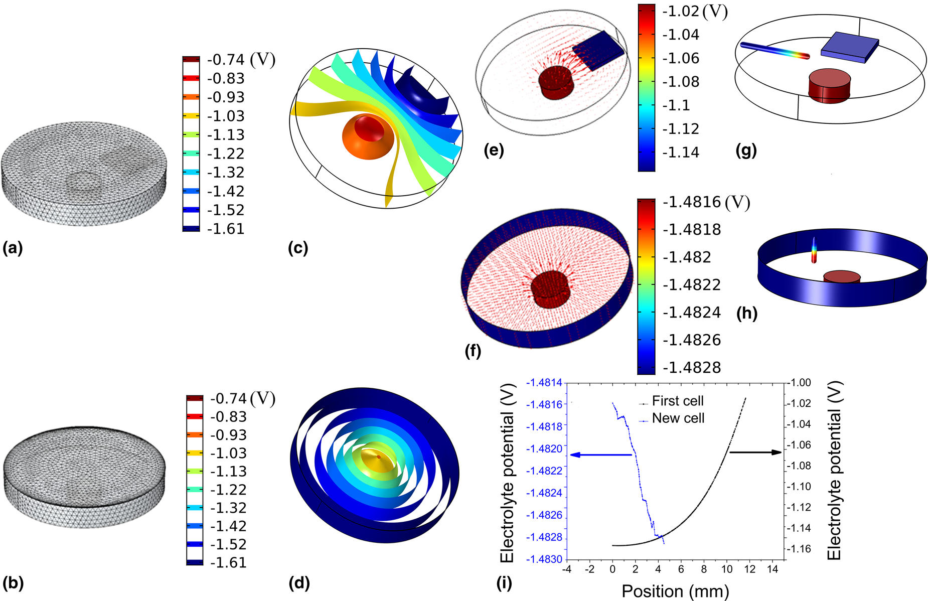
Figure 2: Simulation of the electric field in the two different cell designs. (a and b) The meshing of the cell. (c and d) The equipotential surfaces in the electrolyte for the two different electrochemical cell designs. (e and f) The electrical current vector represented by the arrows in the two cells weighted by their magnitude. The change in the simulated electrolyte potential with the position of the reference electrode is present in (g–i); (g and h) the potential electrode in the two cell designs along the displacement direction of the reference electrode; the color of the axis represents the local electrolyte potential given by the color bar on the right-hand side and (i) the electrolyte potential versus the position inside the electrolyte for the two cell designs.
Potential distribution
To have a better visualization of the potential distribution, the calculated equipotential surfaces in the two cells [Figs. 2(c) and 2(d)] were chosen and plotted. Figures 2(c) and 2(d) clearly illustrate how the electrical potential changes when altering the electrodes’ configuration. In the previous design of cell, the electrical potential distribution is not uniform, in neither the horizontal nor in the vertical plane, as can be seen from Fig. 2(c), while the new design shows a symmetrical distribution of the electrolyte's electrical potential. In the previous design, the equipotential surfaces [Fig. 2(c)] have a semi-parabolic shape around the working electrode in the horizontal plane. In the new design, the equipotential surfaces are concentric cylindrical shells [Fig. 2(d)]. The shape of the cylinders only starts to deform in the vicinity of the working electrode.
Current distribution
The distribution of the electrical current in the two designs is illustrated by plotting the current vector inside the electrolyte, as shown in Figs. 2(e) and 2(f). The distribution of the current inside the electrolyte in the case of the previous design is highly nonuniform [Fig. 2(e)]. The magnitude of the current nearby the working electrode (red) is high, but it starts to diminish as we get closer to the counter electrode (blue), which is represented by the size of the arrow in Fig. 2(e). In the case of the new design, the current lines appear radial, and uniformly distributed on the working electrode (red), whereas at the edge of the working electrode the current has a somewhat larger magnitude [Fig. 2(f)].
Effect of the reference electrode's position on the uncertainty of the measured potential
The reference electrode (RE) is normally used to measure the potential difference between the working electrode and a selected point inside the electrolyte. Ideally, the reference electrode should be positioned in the vicinity of the working electrode to reduce the ohmic loss, and consequently to reduce the uncertainty in the measurement, which can be done in practice by means of a lugging capillary positioned on the surface of the working electrode. Using a lugging capillary is not possible in the case of electrochemical AFM measurements, as it would prevent the AFM scanning head from approaching the surface of the working electrode. Alternatively, the reference electrode can be positioned either outside the cell [Reference Bertrand, Rocca, Savall, Rapin, Labrune and Steinmetz42] or inside the cell to sense the potential [Reference Kreta, Rodošek, Slemenik Perše, Orel, Gaberšček and Šurca Vuk28, Reference Rodošek, Kreta, Gaberšček and Šurca Vuk29, Reference Wanless, Senden, Hyde, Sawkins and Heath35, Reference Schindler and Kirschner36, Reference Surca, Rodošek, Kreta, Mihelčič, Gaberšček, Delville and Taubert41]. In this study, we investigated the uncertainty introduced to the measurements due to the displacement of the reference electrode along the axis of the cylinder shown in Fig. 2(i).
In our new design, the position and orientation of the reference electrode were chosen by taking into account two factors. First, the tip of the reference electrode should be positioned as near as possible to the working electrode, in such a way that its body does not introduce a field distortion. Second, due to the symmetry of the potential distribution within the electrolyte [Fig. 2(d)], the long axis should be oriented in a direction parallel to the equipotential surface [Fig. 2(d)].
Figures 2(g) and 2(h) depict the change in the local potential with the displacement of the reference electrode for the two cells when the cell potential was 0.5 V in both cases. A line was cut in the direction of placing the reference electrode [Figs. 2(g) and 2(h)] to find the local electrolyte potential along the axis of this line. The line is presented using colors, with the colors identifying the local electrolyte potential. The value of the local potential is plotted against the displacement of the electrode [Fig. 2(i)], such that it starts from the body of the cell in the direction of the working electrode in both cases. Figure 2(i) shows that the electrolyte potential changes exponentially by displacing the electrode closer in the case of the old cell and linearly in the case of the new one. When using our previous design, we were trying to place the reference electrode in the vicinity of the working electrode to reduce the error in measuring the electrolyte potential [Reference Kreta, Rodošek, Slemenik Perše, Orel, Gaberšček and Šurca Vuk28]. Therefore, the part of the exponential curve that is in the vicinity of the electrode is fitted to a line. The slope of the line in the case of the old cell is 27.4 mV/mm, while it is 0.43 mV/mm in the second. This can result in an error and makes a comparison between different experiments difficult. This error is greatly reduced in the case of the new design. We can conclude that our approach to positioning the reference electrode in the vicinity of the working electrode and to moving along a direction parallel to the isopotential surface is a valid approach to reducing the uncertainty in measuring the electrochemical potential.
SEM/EDS measurement
Prior to [Fig. 3(a)] and after [Fig. 3(b)] running the electrochemical experiments, the samples were investigated using an SEM. The goal was to find correlations between the morphological and compositional (using EDS) features, on the one hand, and the electrochemical response, on the other hand. From several measurements, we only display the most typical.
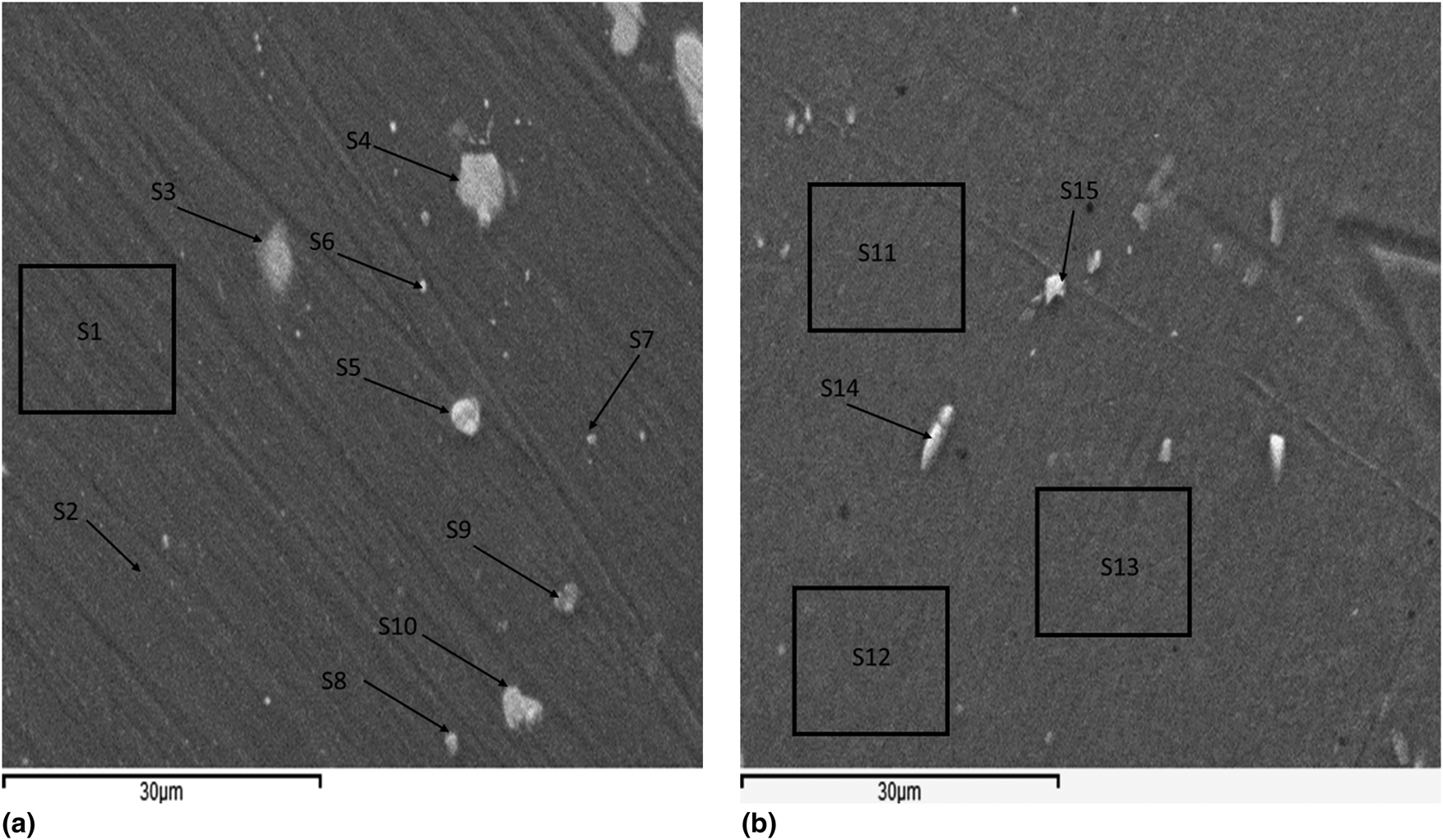
Figure 3: SEM images of a polished AA2024 sample. (a) Before exposure to NaCl and (b) after carrying out EC-AFM and exposure to NaCl. The labeled areas and spots indicate the location of the collected spectra shown in Table 1.
TABLE 1: EDS spectra of AA2024.

Spectra (1–10) before immersion in NaCl, and spectra (11–15) after immersion in NaCl and exposure to different electrochemical potentials. Values are normalized in at.%.
The elemental compositions of the sample are presented in spectra 1–10 (Fig. 3). These correspond to the EDS spectra collected prior to any exposure to NaCl at the locations marked in Fig. 3(a). Whereas the remaining spectra represent the locations marked in Fig. 3(b) after the electrochemical processes described in the section “In situ EC-AFM measurements”. Spectra 1 and 2 reveal the presence of aluminum (more than 90%) and several percentage points of carbon; the rest are traces of Cu, Mg, and Si. In contrast, spectra 3–5 have an interesting feature in common, i.e., in all cases, the ratio of Al:Cu:Mg ~ 2:1:1. This ratio corresponds well to the S-phase of AA2024 Al6CuMg [Reference Boag, Hughes, Glenn, Muster and McCulloch43, Reference Schneider, Ilevbare, Scully and Kelly44, Reference Leblanc and Frankel45, Reference Zhu and van Ooij46, Reference Boag, Hughes, Wilson, Torpy, MacRae, Glenn and Muster47]. In spectra 6 and 7, the ratio Al:Cu is found to be approximately 10:1. Spectrum 8 shows the following ratio of elements: Al:Fe:Mn:Si = ~13:3:3:1, which is close to that of the θ-phase, i.e., Al12(Fe, Mn)3Si. Finally, spectra 9 and 10 show the ratio Al:Cu:Fe:Mn = ~5:1:1:1 [Reference Boag, Hughes, Wilson, Torpy, MacRae, Glenn and Muster47, Reference Buchheit48]. It is clear that oxygen exists in all the spectra of the sample examined before exposure to NaCl with an average of 1.50% atomic ratio. We ascribe this finding to the presence of the native oxide layer. The abundance of different phases depends on the preparation method and the treatment of the alloy. The presence of carbon could be due to either the polishing process or the contamination originating from the exposure to the electron beam. Due to the penetration depth of the X-rays, some observed traces of elements might be associated with the layer(s) underneath the surface. An increase in the ratio of oxygen is noticeable in the EDS spectra measured after the electrochemical process (spectra 11–15) (Table 1). The bright spots from the two spectra 14 and 15 are closer to the composition of the noble phases Al7CuFe2 and Al6MnFe2, respectively.
In situ EC-AFM measurements
The initial scan of the AA2024 sample in air is shown in Fig. 4(a). After the injection of the electrolyte into the cell, the sample was scanned again [Fig. 4(b)]. Comparing the two images in Fig. 4, we see that mostly the same area was scanned in both cases, with a slight lateral shift. This is strong evidence of the mechanical stability of our cell design, which makes it possible to image the selected surface area irrespective of the fluid flow and the application of the electric field.
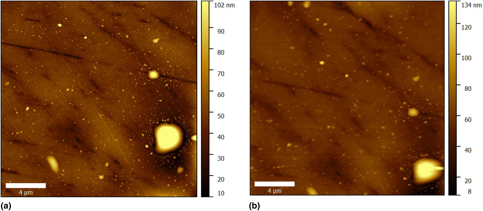
Figure 4: AFM topography images of the AA2024 sample. (a) The sample scanned in the air and (b) the sample scanned immediately after injecting the electrolyte into the cell.
Then, a fresh sample was mounted into the cell and a smaller spot of 10 × 10 μm2 was chosen for the purpose of studying in situ the changes in morphology. Besides monitoring the changes with time, we were particularly interested in changes caused by the application of different values of potential pulses. For this experiment, we used our newly designed electrochemical cell [Fig. 1(b)].
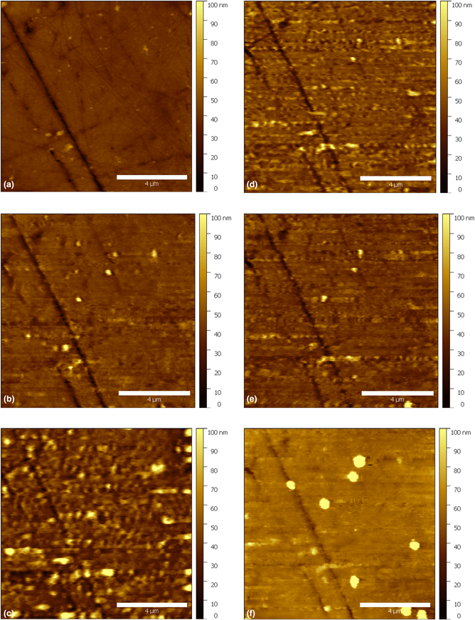
In the first step of the experiment, we simply monitored the development of the open-circuit potential (OCP) without applying any electrical signal [Fig. 5(a)]. Then, still under OCP conditions, the EIS was measured (Fig. 7). Afterwards, chrono-amperometric pulses of different potential values and 20 s duration were applied to the working electrode. We started at −0.8 V/Ag/AgCl/NaCl Satd and ended at a more anodic potential of 0.2 V/Ag/AgCl/NaCl Satd. AFM images were collected after the application of each chrono-amperometric pulse, some of which are presented in Fig. 5. A dramatic change in the surface topography as a consequence of the electrical pulses can be seen in Fig. 5. The measurements were carried out for about 3 h, after which the EIS was measured again at the OCP (Fig. 7). The collected AFM images were used to construct a video so as to visualize the temporal change of the topography with the application of the anodizing potentials (see Supplementary material).

Figure 5: In situ AFM topography measurement of immersed AA2024 with the application of chrono-amperometric pulses: (a) 4 min; OCP, (b) 72 min; −0.3 V, (c) 95 min; −0.2 V, (d) 103 min; −0.1 V, (e) 110 min; 0 V, and (f) 175 min; 0.1 V. Time in minutes refers to the time elapsed after the introduction of 0.5 M NaCl electrolyte. The duration of each chrono-amperometric pulse was 20 s. The images were collected after the application of chrono-amperometric pulses. All the potential values are measured versus a standard Ag/AgCl/NaCl Satd reference electrode. The scale bars are of length 4 μm.
The observed changes were quantified using three statistical surface parameters (roughness root mean square Sq, skewness Ssk, and kurtosis Sku) [Reference Kreta, Rodošek, Slemenik Perše, Orel, Gaberšček and Šurca Vuk28, Reference Surca, Rodošek, Kreta, Mihelčič, Gaberšček, Delville and Taubert41].
The extracted parameters were plotted versus time and the applied potential pulse (Fig. 6). After 4 min of immersion [Fig. 5(a)], the sample's roughness, skewness, and kurtosis were 4 nm, −1.84 and 12.71, respectively. After 10 min of immersion, a chrono-amperometric pulse with an amplitude of −0.8 V/ Ag/AgCl/NaCl Satd and a duration of 20 s was applied to the working electrode. The pulse had a negligible effect on the roughness [Fig. 6(a)], while the skewness [Fig. 6(b)] and kurtosis [Fig. 6(c)] increased, which is evidence of a layer or sublayer growing on the surface. We found that the surface started to shift slightly, and some features appeared to make the surface more asymmetric. After 20 min of immersion, another 20 s pulse was applied to the working electrode; however, this time with an amplitude of −0.6 V/Ag/AgCl/NaCl Satd. A small increase in the roughness, accompanied by a decrease in the skewness and kurtosis were observed. The change of the surface parameters can be correlated with selected features that started to appear in the image. In the next step, a more positive pulse (−0.4 V/Ag/AgCl/NaCl Satd) of 20 s was applied, which caused a slight increase in the roughness (from 4 to 5 nm), with a simultaneous increase in both the skewness (from −0.1 to 1.39) and kurtosis (from 20.63 to 23.50). After 52 min of immersion, a −0.3 V/Ag/AgCl/NaCl Satd pulse was applied to the working electrode while imaging. It was found that the roughness started to increase rapidly, although no potential was applied during the next 30 min. The roughness reached a value of 9 nm, the skewness increased noticeably, while the kurtosis started to decrease. The roughness attained its maximum value (18 nm) upon the application of −0.2 V/Ag/AgCl/NaCl Satd after 88 min of immersion. That increase in the roughness could be correlated with the evolution of selected features on the surface. Since the electrolyte used has a neutral pH, the increased roughness, which is clearly present in Fig. 5(c), must be due to the formation of an amorphous oxide/oxyhydroxide layer [Reference Alwitt7, Reference Thompson12]. With the application of a −0.1 V/Ag/AgCl/NaCl Satd pulse for the second time at 103 min of immersion [Fig. 5(d)], the roughness started to decrease. This trend continued during the next step as well, i.e., with the application of 0 V/Ag/AgCl/NaCl Satd [Fig. 5(e)]. Then, with the application of more positive pulses, specifically 0.1 V/Ag/AgCl/NaCl Satd, the surface roughness started to increase as well as the kurtosis and skewness (Fig. 6). As shown in Fig. 5(f), the features on the surface have a larger size than the initial one [Fig. 5(a)]. Thus, it is clear that the surface looks smoother in Fig. 5(f) than before [Fig. 5(d)]. The increased size of the features appeared to have a significant effect on the increasing roughness and the other parameters. The increase of the features’ sizes on the surface could be either due to the change in the tip geometry,or a change in the feature surface. Since the AFM tip could resolve some small particles on the surface in the last image, that means the AFM tip was relatively sharp. After 180 min of immersion, an EIS spectrum was acquired (Fig. 7). The acquired spectrum showed an increase in the impedance.

Figure 6: Time dependence of the surface parameters for an electric potential applied to AA2024 in NaCl (0.5 M). (a) The surface roughness RMS, (b) the surface kurtosis, (c) the surface skewness, and (d) the applied potential pulse value with time (the duration of each pulse is 20 s). The arrows indicate the images selected and presented in Fig. 5.

Figure 7: In situ EIS measurements of AA2024 measured before and after applying chrono-amperometric pulses. (a) Nyquist plot (b) Bode plot of EIS was measured before (black curve) and after (red curve).
Therefore, that change of the surface topography, accompanied by an increase in the electrochemical impedance, was due to the formation of a pseudo-boehmite layer [Reference Hart9, Reference Kreta, Rodošek, Slemenik Perše, Orel, Gaberšček and Šurca Vuk28, Reference Kreta49]. This was already proven in our previous infrared reflection-absorption study [Reference Kreta, Rodošek, Slemenik Perše, Orel, Gaberšček and Šurca Vuk28].
The newly designed cell [Fig. 1(b)] made possible measurements of the topography by locating the same spot in the air and after injecting the liquid into the cell (Fig. 4), with only a slight drift during the course of the experiment (3 h), as shown in Fig. 5. The advantage of this cell over our previous design [Fig. 1(a)] is that it can carry out different electrochemical measurements (e.g., chrono-amperometric and EIS) simultaneously by scanning the surface topography. Thus, the symmetry of the field distribution within the electrolyte together with choosing the pulse duration (20 s) reduced the evolution of gas bubbles that were obstacles to the AFM tip with the previous cell [Reference Kreta, Rodošek, Slemenik Perše, Orel, Gaberšček and Šurca Vuk28, Reference Surca, Rodošek, Kreta, Mihelčič, Gaberšček, Delville and Taubert41]. Typically, the new cell allows controlling, monitoring, and measuring electrochemical events, while monitoring the change of topography. The cell is easy to use and maintains the field symmetry, which ensures the repeatability of the experiments.
Conclusions
A comparative study showed the effect of electrode geometry and arrangement on the uniformity of current and voltage distributions in an electrochemical cell intended for in situ AFM measurements. 3D FEM simulations showed that the newly proposed cell design had a much more uniform current and voltage distribution in the electrolyte than an earlier design. The selection of the reference electrode in the new design can reduce the uncertainty of displacing it by a factor of 60 times less than our previous design. It was proven that an in situ AFM could follow the changes in the topography to elucidate the growth of an oxyhydroxide layer upon the application of anodizing potentials. By combining the AFM and in situ EIS before and after the measurements, we confirmed the change in the surface due to the growth of the oxyhydroxide layer. The SEM/EDS showed an increase in the oxygen contents on the surface due to the growth of the oxyhydroxide layer. Finally, we can conclude that the newly designed electrochemical cell allowed the use of different electrochemical techniques (EIS and chronopotentiometry), while monitoring the surface's topography, simultaneously.
Experimental
Material
Aluminum alloy AA2024-T3 sheet of 4 mm thickness (Goodfellow, UK) was cut into 7-mm-diameter disks and prepared for in situ and polished as described elsewhere [Reference Kreta, Rodošek, Slemenik Perše, Orel, Gaberšček and Šurca Vuk28]. An Ag/AgCl/0.3 M NaCl reference electrode (BASi) was used, and 99.99% platinum foil of 0.5 mm thickness (Sigma-Aldrich, Taufkirchen, Germany) was cut and formed as a cylindrical shell counter electrode. Sodium chloride electrolyte of 0.5% molar concentration was prepared using NaCl purchased from Sigma-Aldrich that it was dissolved in deionized water (18.2 MΩ cm Milli-Q water).
Electrochemical cell simulation and design for in situ measurements
3D Simulation of electric field distribution in electrochemical cells
The symmetry of the electric field distribution is an important factor in an electrochemical cell, as it is correlated with the uncertainty of the electrochemical measurements. For example, the distribution of the current lines can critically influence the electrochemical processes in the cell. More specifically, the area of the electrode that has a higher current density can become more prone to degrade faster than its corresponding area with a lower current density. In many electrochemical systems, knowledge of the current density distribution can be used for either minimizing the error in the measurements or minimizing the unwanted effects, such as inhomogeneous deposition in the case of electrochemical deposition, and the inhomogeneous degradation of electrodes.
The motivation for the new design was to be able to simultaneously measure the change in the surface topography and the electrochemical impedance under potential control with a reduced uncertainty. The purpose of simulating the electric field distribution in the electrochemical cells is to find how the electrical currents and potentials are distributed inside the electrolyte, and how they change when changing the electrode configuration before manufacturing the newly designed cell. A comparison between our previous cell [Fig. 1(a)] and the newly designed cell [Fig. 1(b)] will highlight the effects of the cell and electrode geometries on the distribution of the electric field inside the cell.
In the case of using a finite-element method (FEM) simulation, a set of differential equations is solved using the FEM. By defining the boundary conditions for each geometry, the solution can be determined. A three-dimensional simulation is carried out using standard finite-element software (COMSOL Multiphysics™) [Reference Dickinson, Ekström and Fontes50].
Physics of simulation
First, the geometry of each cell is modeled in 3D, as illustrated in Figs. 1(c) and 1(d), such that the electrolyte is represented as a cylinder that has boundaries with both the anode and the cathode. The working electrode only contacts the electrolyte on one surface, while the counter electrodes are simulated by two metals contained inside the electrolyte cylinder, which has a rectangular shape in the first design and a cylindrical shell in the second design.
The aim of this simulation study was to investigate the effect of the electrodes’ arrangement and their geometry on the symmetry of both the current and the potential distribution within the electrolyte. There are three different schemes of current distribution in the electrolyte: primary, secondary, and tertiary [Reference Newman and Thomas-Alyea51]. In our study, we were interested in studying the primary current because it depends solely on the geometry of the electrodes and their arrangement [Reference Newman and Thomas-Alyea51]. Fast kinetics is assumed in the case of the primary current distribution, which conveniently leads to a simplification whereby the potential of the electrolyte adjacent to the electrode equals that applied to the electrode. The primary current distribution is governed by Ohm's law [Eq. (1)], which only depends on the electrolyte's conductivity (σ) and the potential (φ) gradient. The potential distribution fulfills the Laplace equation [Eq. (2)]. The FEM is used to solve these two differential equations at points distributed within the electrolyte through a mesh, which is described below. The boundary conditions are used as mentioned above: the electrolyte potential equals that applied to the metal electrodes. To find the field distribution, we assume that the working electrode is the anode and the counter electrode is the cathode. The system is described with the following equations:
 $${\bi J} = -{\rm \sigma }\nabla {\rm \varphi }$$
where J is the current density (A/m2), σ is the electrolyte's conductivity, and φ is the potential in the liquid.
 $$\nabla ^2{\rm \varphi } = 0$$
The cathode potential was chosen to be zero (V C = 0) since the potential of the electrode equals the potential difference between the electrode and the ionic potential of the adjacent liquid.
Since the kinetics is fast, the equilibrium potential V eq equals the potential difference between the solid phase potential of the cathode (V C) and the adjacent electrolyte potential φC, which implies that
 $$V_{{\rm eq}}\lpar {{\rm cathode}} \rpar = V_{\rm C}-{\rm \varphi }_{\rm C} = -{\rm \varphi }_{\rm C}$$
Since the cell potential is the potential difference between the anode (V A) and the cathode (V C) potentials
 $$V_{{\rm cell}} = V_{\rm A}-V_{\rm C} = V_{\rm A}$$
 $$V_{{\rm eq}}\lpar {{\rm anode}} \rpar = V_{\rm A}-{\rm \varphi }_{\rm A} = V_{{\rm cell}}-{\rm \varphi }_{\rm A}$$
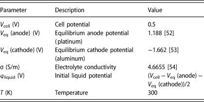
All the parameters and the initial values are listed in Table 2.
TABLE 2: Parameters used in the simulation.
Meshing
After setting all the physical parameters of the simulation, the meshing had to be setup. In a finite-element simulation, the meshing step is a critical point, as poor meshing parameters lead to unreliable results. The meshes were chosen in such a way that the boundaries between the electrodes and the electrolyte interface meshed with a very fine thickness of 20 nm, which means that 392,000 elements were used in the meshing of each cell. Figures 2(a) and 2(b) show the concept of meshing for the cells.
Cell design
In the case of designing an electrochemical cell for the scanning probe microscopy (SPM) measurements, many factors had to be considered. The main problem is the space constraint, which is common to all AFMs. The electrode arrangement is important since an inappropriate arrangement can introduce uncertainty and/or distortion [Reference Klink, Madej, Ventosa, Lindner, Schuhmann, La Mantia and La55, Reference Delacourt, Ridgway, Srinivasan and Battaglia56] to the electrochemical measurements.
The previous cell [Fig. 1(a)], which is used here as a reference cell, was designed for in situ AFM measurements of corrosion—either spontaneous or under potential control [Reference Kreta, Rodošek, Slemenik Perše, Orel, Gaberšček and Šurca Vuk28, Reference Rodošek, Kreta, Gaberšček and Šurca Vuk29, Reference Mihelčič, Surca, Kreta and Gaberšček40, Reference Surca, Rodošek, Kreta, Mihelčič, Gaberšček, Delville and Taubert41]. The first problem with this asymmetric design [Fig. 1(a)] was that the scanning head of the AFM had to be removed to inject the solution into the cell. Additionally, the arrangement of the electrodes could change from one measurement to another. The latter can result in an error in the measurements or can make a comparison between different samples less reliable. In the new symmetric design [(Fig. 1(b)], two liquid ports were added, which means the cell can be used as a flow cell. In addition, the counter electrode was made of a platinum sheet formed as a cylindrical shell to surround the working electrode to preserve the field symmetry; therefore, a more uniform current distribution can be attained. In contrast to our previous design, the reference electrode is placed vertically for different reasons: first, it facilitates maneuvring the AFM head in the cell; second, it disturbs the current distribution to a lesser extent (as elaborated in the simulation section “Effect of the reference electrode's position on the uncertainty of the measured potential”); and, finally, it helps avoid the contaminations that can result from the reference electrode. Such a design is easy to fit into the microscope, it facilitates the connection of the electrodes and makes it possible to keep the microscope box closed during the experiment and thus reduce the mechanical noise. However, our main concern was whether such a design was able to keep the field distribution symmetric. This problem was solved and the field distribution preserves a high symmetry, which is further presented and elaborated in the simulation section “Simulation” below. The inner diameter of the newly designed cell is 32 mm, and this can accommodate samples of different diameters up to 9 mm. In addition, it supports a standard reference electrode to reduce the uncertainty of the potential measurement. The electrodes are then connected to an external potentiostat using a coaxial cable to reduce the electrical noise. Using this design, it is guaranteed that the position of the electrodes will not change from one experiment to another, which significantly contributes to the repeatability. The cell can be used either as a flow cell or a constant-volume cell. In the former case, a pump is remotely connected to the inlet and outlet liquid ports, while in the latter one, port is closed and the electrolyte is injected into the cell using a syringe through a silicon tube.
The most common materials used in the production of electrochemical cells are glass, such as Pyrex [Reference Deyab57] and quartz [Reference Schindler and Kirschner36], or polymers, such as Kel-F [Reference Bertrand, Rocca, Savall, Rapin, Labrune and Steinmetz42] and Teflon [Reference Mišković-Stanković, Jevremović, Jung and Rhee58, Reference Davoodi, Pan, Leygraf and Norgren59, Reference Li and Lampner60]. Obviously, on the one hand, glasses have a high service temperature, and they have outstanding toughness compared to polymers. On the other hand, polymers have superior electrical resistivity and are resistant to most chemical compounds. In our case, Teflon was the most appropriate material for the cell's construction based on the following advantages: ease of fabrication, low cost, high electrical resistivity, chemically inactivity toward mild and most harsher chemicals, and ease of cleaning.
The base of the cell was made of steel, so that it could be attached to the magnetic base of the microscope. The final design of the cell was made in three dimensions using a CAD program and exported as a binary file to a computer numerical controlled (CNC) milling machine, where it was fabricated.
In situ EC-AFM measurements
An Agilent AFM 5500 was used for the in situ measurements. Four-sided (pyramidal) silicon tips with the radius less than 50 nm (Nanosensors) were used, gold coated on a detector and a tip side, with a nominal spring constant of 0.1 N/m, a resonance frequency of 75 kHz in the air and a cantilever length of 200 μm.
The in situ AFM measurements were carried out in the tapping mode, so that the repositioning of the corrosion features during imaging as well as reducing the lateral forces could be avoided. The images were collected at a scanning rate of 2 Hz with dimensions of 10 × 10 μm2.
Before performing the measurements using the electrochemical cell [Fig. 1(b)], the cell was washed using a detergent in tap water and then carefully rinsed with deionized water. Afterwards, it was sonicated twice in deionized water for 30 min, and then sonicated in acetone for degreasing and finally in acetone, for 30 min each time. Finally, it was sonicated in Milli-Q water (18.2 MΩ cm) for 30 min. Next, the sample was mounted in the center of the cell. To have a robust electrical contact with the conductor fixed at the bottom of the cell, a conducting colloidal silver paste was added below the sample (between the sample and the conductor at the bottom), which ensures the electrical connectivity to the wire-connected potentiostat and makes the sample mechanically fastened. The sample height was adjusted to make sure it was at the same level as the base of the cell. Paraffin wax was applied to the perimeter of the sample, so that the edges of the sample were covered and appropriately anchored in the sample [Reference Kreta49]. The cell was then attached to the microscope and the three electrodes were connected to a Bio-Logic SP-200 (Bio-Logic SAS, Claix, France) potentiostat to make the electrochemical measurements. Afterwards, the electrolyte was injected into the cell. The cantilever's oscillation frequency was tuned and approached the sample's surface. After 30 min of immersion, EIS was conducted at the OCP using a sinusoidal potential signal of 5 mV amplitude in the logarithmically spaced frequency range from 7 MHz to 0.1 Hz. Then, the sample surface was scanned continuously for about 3 h with the application of chrono-amperometric pulses from the cathodic potential (−0.8 V/Ag/AgCl/NaCl Satd) to the anodic potential (0.2 V/Ag/AgCl/NaCl Satd). After that, the EIS was measured again, before removing the tip and the electrolyte. After the experiment, the collected images were processed to extract the statistical parameters (roughness root mean square Sq, skewness Ssk, and kurtosis Sku) using a previously developed Matlab script [Reference Kreta, Rodošek, Slemenik Perše, Orel, Gaberšček and Šurca Vuk28, Reference Surca, Rodošek, Kreta, Mihelčič, Gaberšček, Delville and Taubert41].
SEM/EDS measurements
The SEM micrographs of the samples before and after the immersion were recorded on a Supra 35 VP (Carl Zeiss) field-emission scanning electron microscope (FE-SEM) equipped with an INCA 400 (Oxford Instruments). The EDS sensor was of an emergency type with an area of 10 mm2. The corroded samples were first dried using a gentle flow of nitrogen and then kept in a dry box for a day before inserting them into the SEM. The samples were mounted on aluminum stubs using the carbon tape to avoid any charging of the samples. The micrographs and EDS spectra were collected at an accelerating voltage of 10 kV.
Data availability
The raw/processed data required to reproduce these findings cannot be shared at this time as the data is a part of an ongoing study.
Declaration of competing interest
The authors declare that they have no competing financial interests or personal relationships that could have influenced the work reported in this paper.
Acknowledgments
A.K. appreciates the financial support [project number H017002] of the Slovenian research agency for his Ph.D. The authors are grateful to COMOSL for allowing them to use a trial version.
Supplementary material
To view supplementary material for this article, please visit https://doi.org/10.1557/jmr.2020.275.


 Open access