
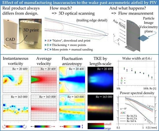
Effect of Manufacturing Inaccuracies on the Wake Past Asymmetric Airfoil by PIV


1
Faculty of Mechanical Engineering, University of West Bohemia, Univerzitní 22, 306 14 Pilsen, Czech Republic
2
Institute of Thermomechanics, Czech Academy of Sciences, Dolejškova 5, 180 00 Prague, Czech Republic
*
Author to whom correspondence should be addressed.
Energies 2022, 15(3), 1227; https://doi.org/10.3390/en15031227
Submission received: 2 December 2021
/
Revised: 20 January 2022
/
Accepted: 31 January 2022
/
Published: 8 February 2022
(This article belongs to the Special Issue Investigation, Optimization, and Discussion of Turbulence)
Abstract
:The effect of manufacturing geometry deviations on the flow past a NACA 64(3)-618 asymmetric airfoil is studied. This airfoil is 3D printed according to the coordinates from a public database. An optical high-precision 3D scanner, GOM Atos, measures the difference from the idealized model. Based on this difference, another model is prepared with a physical output closer to the ideal model. The velocity in the near wake (0–0.4 chord) is measured by using the Particle Image Velocimetry (PIV) technique. This work compares the wakes past three airfoil realizations, which differ in their similarity to the original design (none of the realizations is identical to the original design). The chord-based Reynolds number ranges from to . The ensemble average velocity is used for the determination of the wake width and for the rough estimation of the drag coefficient. The lift coefficient is measured directly by using force balance. We discuss the origin of turbulent kinetic energy in terms of anisotropy (at least in 2D) and the length-scales of fluctuations across the wake. The spatial power spectral density is shown. The autocorrelation function of the cross-stream velocity detects the regime of the von Karmán vortex street at lower velocities.
1. Introduction
Fluid flow is a highly non-linear problem that still lacks a reasonable solution. One of the general effects of non-linearity is the unpredictable response to even small perturbations or changes of the boundary conditions. The scale of possible responses to a small geometry perturbation ranges from almost zero effect to a linear response and up to a complex change of flow state. The famous butterfly effect represents this behavior with the example of a small butterfly that can alter the evolution path of a turbulent system [1]. As there is a large number of such micro-events, the evolution path of the entire system is unpredictable. However, the statistical properties can be predicted quite reasonably. This feature is used in modern computational fluid dynamics, which does not solve the non-linear Navier–Stokes equations on a fine mesh with the resolution of the Kolmogorov length-scale, but it solves only much larger cells with a direct link to the geometry of the boundary conditions under the assumption that the behavior at smaller scales follows some of the turbulence models.
The relatively low-cost computational fluid dynamics are used in thorough experiments in the area of industrial design and optimization. However, the computational methods need validation and verification [2], which are mainly based on the comparison with an appropriate experiment, which does not need to fit in all parameters, but at least the main geometrical and fluid properties might be met. This is where the problem with geometry becomes important—the object used in the experimental study is different from the desired design used in the computational approach. As the quality needs to increase, even smaller deviations between numerical and experimental results can be accepted. As the experiment has a semblance of truth, mathematicians have devoted a great deal of effort to developing even better and more accurate models in order to fit the experimental data measured with boundary conditions that are known only approximately.
In this study, we used a high-quality, contactless 3D optical scanner to measure the real geometry of boundary conditions (of course, with some uncertainty connected with each measurement technique) and compare the flow field past an airfoil produced at three levels of accuracy—the first variant represents the naive approach, and we sent to the 3D printer only the coordinates obtained from a public database [3]. If we had not used a 3D optical scanner, our study would have ended by declaring “we measured flow in the near wake past airfoil…”. However, the 3D scan discovered discrepancies from the ideal geometry, and therefore we attempted to prevent these by manipulating the geometry in such a way that the outcome could be brought closer to the ideal case. This step was repeated creating two more variants that were increasingly close to the ideal geometry. In any case, the best product was still different from the ideal geometry used in the processes of numerical optimization.
There are only very few other studies about manufacturing inaccuracies, and they are numerical only. Our study is experimental and compares models that have been actually created. A disadvantage of this work is that the ideal geometry does not exist in reality; hence, we can compare only different levels of manufacturing attention.
Some Recent Literature Concerning This Problem
Moreno-Oliva and coworkers [4] used the Laser Triangulation Technique to measure the real profile of a NACA0012 and FX 61-137 airfoil; one realization of the NACA0012 has been commercially made of metal, while the second has been 3D printed by the authors from PLA, and the profile FX 61-137 was measured at the real wind turbine blade at several heights. They used the measured profiles as an input for the Xfoil software [5] together with the theoretical profiles. They report a significant decrease of performance of the real wind turbine profiles when compared with the ideal geometry.
Ravikovich et al. [6] performed an optimization of fan blades with real geometry deviations from airfoil geometry. Their algorithm simultaneously solves mechanical integrity problems and the aerodynamic stability of the flow. The geometry data measured under cold conditions are transformed via numerical simulation into hot conditions, which allows the estimation of the influence of the measured geometry on the final fan parameters.
The effect of even small geometry modifications in turbine stator blades was studied by Klimko and Okresa [7]. Modifications in the stator wheel affect the reaction and efficiency of the entire stage. Data like those mentioned above are used in the numerical optimization [8] of the developed new stage.
Winstroth and Seume [9] studied numerically the effect of several artificial geometry deviations on four wind turbine airfoils. The geometry deviations cover mold tilt towards the leading or trailing edge, step changes at certain positions, sine waves placed at several positions on both pressure and suction sides or at the leading edge, and the thickening of the profile—in total, 40 modifications of four different airfoil profiles are used in the studied wind turbine. They found that the worst deviation (in terms of energy production) is the tilt towards the leading edge; they found also some cases with a positive impact.
The structure of our article is as follows: first, we describe the methods including 3D printing, 3D optical scanning, and Particle Image Velocimetry used to measure 2D velocities within a square area past the trailing edge. This paper focuses on data at zero angle of attack; some data at an angle of attack of are in the Appendix A. The ensemble average stream-wise velocity, the path of the wake centerline, and the wake width based on the average stream-wise velocity are shown. The lift coefficient is impossible to determine on the basis of PIV data; therefore, a simple balance is introduced and the lift at zero angle of attack and at several Reynolds numbers is measured. The turbulent kinetic energy is explored to discuss if it is produced by fluctuations in the stream-wise or cross-stream velocity component. The length-scale of fluctuations is explored by a unique method developed at the University of West Bohemia in Pilsen. The autocorrelation function reveals the periodicity at low velocities and the decay of the integral length-scale at larger ones.
2. Materials and Methods
2.1. Three-Dimensional Printer
We used a commercially available 3D printer Prusa Mk 2.5. It uses the FDM (Fused Deposition Modeling) printing technology [10]. The used material is thermoplastic polymerized lactic acid (PLA) [11]. The nozzle temperature was , and the height of a single layer was . The 3D printed airfoils are used mainly for testing and development purposes. At the current stage, 3D printing technology is not suitable for industrial manufacturing. However, it is important to know the impact of the typical 3D printing shortcomings.
2.2. Three-Dimensional Scanner
The optical 3D scanning method FPS (Fringe Projection Scanning [12]) is based on projecting light periodic stripes onto the surface [12,13], and the variations of their phase are used to estimate the variations of height across the measured surface. The commercial 3D optical scanner GOM Atos Core [14] is used in our study. Mendřický [15] measured the accuracy of a such scanner dependent on the calibration and the optical matteness of the measuring surface of standard spheres. He found that the accuracy is on the order of micrometers, and a matte coating adds around , while simply an old calibration can change the measured results systematically by around . Li et al. [13] found that ambient light has only a small effect on the results, while Vagovský et al. [16] states that even the size of the scanned object influences the accuracy due to the focus blur. The measuring volume of our scanner is ; thus, the airfoil of height is small for such a volume, but still, our object size is much closer to the measured volume than in the case explored by Vagovský [16]. We did not use the matte coating because we used white PLA material; on the other hand, we had to paint the material black before the PIV measurement, which uses intense laser light, and we did not measure the thickness added by this painting.
2.3. Model
The coordinates of the NACA 64-618 airfoil were obtained from the public database Airfoiltools.com [3]. This airfoil is frequently used at the tips of the wind turbines [17] and has a reasonable lift even at high angles of attack (which is valid only for larger Reynolds numbers, as shown later). The trailing edge of this airfoil is sharp, and it points towards the high pressure side; see the black line in Figure 1. First, this airfoil was 3D printed only according to the point coordinates obtained from the public database [3]; this first naive realization is denoted A. Then, a high-precision 3D optical scanner GOM Atos [18] is used to measure the deviation from the ideal geometry; see Figure 1. There exists a huge systematic printing error—the missing trailing edge; see Figure 1c. This is caused by the finite thickness of the extrusion line, which does not fit into the very thin walls, and the program for generating the g-code does not allow the extruder to move into that location. The trailing edge is shorter by almost , which is of the chord length.
A next step was to make the trailing edge thicker in order to fill it with at least some material. This was performed by the Minkowski sum [19] of the airfoil profile with a circle of radius . This method led to an overly large thickening of the entire model, but the trailing edge was still shorter than it should be. This blind method is not reported here. The next trial, denoted B, was performed by artificial manipulation with the profile points at the trailing edge combined with the Minkowski sum with a circle of radius . Now, the trailing edge was shorter by around only. On the other hand, the trailing edge displayed a large radius of around .
The best result was obtained by using the Minkowski sum with circle of radius, adding new points into the trailing edge area and expanding it over the ideal edge. After printing, the model was polished manually in order to sharpen the trailing edge. As a side effect, the surface of this last realization, denoted C, was smoother than the previous ones. The problem with manual polishing is that (i) it is a non-repeatable procedure, and (ii) it is too expensive for possible industrial use.
2.4. Wind Tunnel
The University of West Bohemia in Pilsen has multiple wind tunnels [20,21]. However, due to the laser safety requirements, we are limited for the use of the PIV method to the “small” wind tunnel [22] with a transparent test-section of length and cross-sectional size of . It is an open low-speed wind tunnel driven by a radial fan at the tunnel inlet. The smallest stable velocity used in this study is ; the largest used reference velocity is . The working fluid is atmospheric air with a temperature of around , and the actual humidity was not measured.
The Reynolds number used in this study was based on the above-mentioned reference velocity , which fits the incoming velocity in the case of an empty test section of the wind tunnel. As the length-scale for the Reynolds number, the planned chord length of the airfoil was used. It was a constant: . Note, the real chord length slightly differed among realizations A, B, and C (see Table 1 for more details). The range of Reynolds numbers used in this study spanned one order of magnitude from (corresponding to ) up to , where .
2.5. Particle Image Velocimetry
The method of Particle Image Velocimetry [23] visualizes the wake structure in a small area just behind the airfoil; see Figure 2a. This method is based on the optical observation of the movement of small particles carried by the studied fluid. In our case, the particles are droplets of Safex with a diameter in the order of micrometers. When the droplets are small enough, they follow the fluid motion because the inertial forces scale with particle volume—i.e., as —while the viscous forces unifying the motion of particles and fluid scale with the particle surface—i.e., as . These particles are illuminated in a single plane by using a solid-state pulse laser, New Wave Solo, using the second harmonics of wavelength (corresponding to a green color). The single shot energy is , and its duration is ; thus, the peak power is . The laser produces a pair of pulses separated by tthe ime-interval dependent on the flow velocity. The laser beam is defocused by using cylindrical optics in order to illuminate the plane. The camera is oriented perpendicularly to this plane and focused into it. The Mk II Flow Sense CCD camera has resolution of pixels; this camera is able to resolve both pulses of the laser into a pair of expositions. The obtained pairs of photographs of particles are processed by using the Dantec Dynamic Studio software (details for readers familiar with this software: (1) first five frames are removed from each movie, (2) the minimum of image ensemble is calculated by using Image Min/Max function, (3) this minimum is subtracted from each image in the ensemble by using the Image Arithmetic function, (4) the velocity vectors are calculated by using the Adaptive PIV function with parameters: grid step size 32, minimum IA size 32, maximum IA size 32, validation based on universal outlier detection over neighborhood , normalization , acceptance limit ; the algorithm adapts to the particle density with a particle detection limit of 5 to the desired number of 10 particles per IA; it adapts the IA shape to velocity gradients with and , the convergence limit is pixel and the maximum number of iterations is 10. (6) The last step within the Dantec software is exporting via the Numeric Export function). The vector fields contain vectors, where a single grid point covers an area of corresponding to times the chord length c. The analysis continues by using our custom-made software: one grid point is removed from each side, obtaining vectors with a resolution of , because the vectors at the edge of the field of view are not trustworthy, as there is a relevant number of particles leaving or entering the field of view during the time between laser pulses. The second step is to filter out the snapshots, whose small-scale energy content is significantly greater than the average of the ensemble. This procedure serves to remove rough errors, whose smallest-scale energy content is typically large. This method is described in more detail in our previous article [24]. In fact, the current data have reasonable quality; therefore, this procedure removes at least one snapshot only for 40% of datasets. An example of the obtained instantaneous velocity field is displayed in Figure 3.
2.6. Lift Force Measurement
Wind-tunnel balance is designed to measure the lift force L on the airfoil. The basis of the balance is a resiliently suspended movable table. Elastic suspension is created with four parallel flexible elements. The elastic suspension has the lowest stiffness in the direction of the force L, and in all other directions, the stiffness is an order of magnitude higher. The displacement of the table is measured by an eddy-current sensor that responds to the distance to the steel target. Unwanted vibrations are dampened by eddy-currents in the copper sheet as it moves near to the neodymium super magnet. The output of the sensor is calibrated by a known force created by using a calibration weight in the lift direction.
3. Results and Discussion
3.1. Zero Angle of Attack—Average Velocities
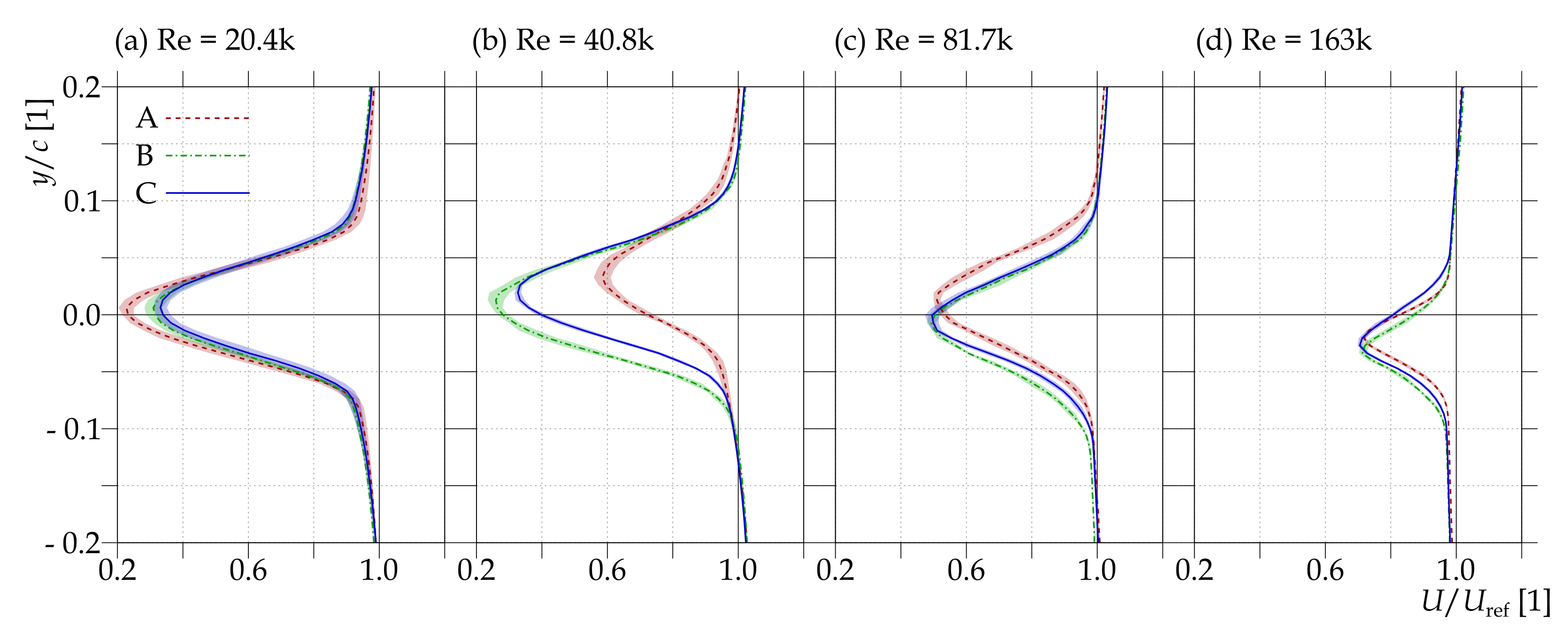
The average stream-wise velocity component for four different Reynolds numbers is displayed in Figure 4. In that figure, the spatial distribution for each case (velocity and airfoil realization) is plotted as a colormap. The direct comparison of isotachs (contour lines of velocity) for each product is plotted in a single panel in order to see the differences between those products. Figure 5 shows the profile of the average stream-wise velocity at distance past the trailing edge. This plot contains less information than the previous one, but this information is organized in a different manner in order to show the differences better.
A first look at Figure 4 and Figure 5 reveals that the largest difference occurs at a Reynolds number of (denoted 40.8 k, where k represents as a standard multiplicator of the SI system). This Reynolds number is close to the critical Reynolds number of transition between a wake dominated by the von-Kármán vortex street [25] and the wake dominated by continuous boundary layers developed along the airfoil, as will be apparent from the next figures analyzing turbulent kinetic energy (mainly the ratio in Figure 6). As was mentioned above, variant A is slightly smaller than B and C, and both are expanded by the Minkowski sum with a circle of radius . Therefore, it is natural to expect that the real Reynolds number for those variants is slightly larger than that for variant A; thus, the transition occurs at slightly smaller velocities.
The next largest discrepancy lies in the position of the wake past variant A. It is most apparent at a Reynolds number of , although it applies at others as well. This shift is caused by the missing trailing edge of the variant A; see Figure 1. As the trailing edge is slanted towards the pressure side (direction down in the figures), the entire airfoil ends at the top (in figures), and thus the entire wake is shifted up. It is even more apparent in the velocity profiles in Figure 5 and Figure 7. One may ask why this shift is less apparent at the lower Reynolds number—we think that this is due to the different mechanism of wake creation: the von Kármán vortex street is formed due to Kelvin–Helmholtz instability of the shear layer between the fluid, which passes far from the obstacle, and between the fluid, which is slowed by the presence of the obstacle. However, this difference starts at the leading edge, which is much more similar for different airfoil variants; see Figure 1b.
3.2. Balance Measurement of Lift Coefficient
According to the momentum balance principle, the lift force acting in one direction has to deflect the fluid motion in the opposite direction. However, the true integration of the deflected momentum requires the knowledge of the flow field around the entire airfoil, which is not available. In order to obtain some information about the lift, which is in any case the crucial feature of any airfoil, we measured this by using a force balance equipped with four flexible metal elements in order to allow deformation in a single direction only; see Figure 8. The resulting lift coefficient is shown in Figure 9 for an angle of attack equal to and for Reynolds numbers in the same range as used for the PIV measurement. This figure shows a reasonable match with the prediction by the Xfoil algorithm [5,26,27] at a Reynolds number of , but the values are greatly different at lower and higher velocities. Differences among airfoil realizations show that the A variant exhibits the lowest lift, as expected. The geometrically best airfoil C has the best aerodynamic performance. Interestingly, the A airfoil has larger negative values of lift at low velocities. The large errors reported here are caused by the unwanted oscillations at higher velocities (despite the damping by using highly-conductive cooper and a strong magnet). At smaller values, a large error is caused simply by the uncertainty of the displacement sensor and of the analog–digital converter, because the forces are two orders of magnitude smaller than the range adapted to fit the expected forces at largest velocities.
3.3. Rough Estimation of Drag Coefficient
The time-average drag force can be roughly estimated according to the principle of momentum balance:
where is the velocity in the unperturbed state—see the work of Terra et al. [28,29] for more details; is the surface element across the wake, and is the variation of u. This fluctuation term originates from the averaging of the Reynolds-decomposed momentum balance equation, and it decreases the resulting force. The calculation of the last term with static pressure p is rather complicated [30], as all components of the velocity gradient are needed to be known in order to integrate the pressure Poisson equation [31]. Terra et al. [28] used tomographic PIV in order to obtain this term, and they found that, fortunately, the pressure term is important only up to the recirculation zone, and it disappears downstream; see Figure 13 in [28]. This observation allows us to ignore this term and estimate the drag force only by using the measured spatial velocity distribution as
where the integration is performed along the y-direction in the measured two-dimensional FoV at a fixed x-position, which is far enough to ignore the pressure term. In our case, is chosen (i.e., the most downstream position within our FoV). H is the height of the prismatic airfoil. The background velocity is replaced by the background of the Gaussian fit of the velocity profile (Equation (5)).
There is another approach to estimate the drag coefficient by using the spatial distribution of the measured velocity across the wake. Antonia and Rajagopalan [32] offer an alternative procedure including the transverse velocity fluctuations as well:
The fluctuations in the stream-wise direction are thought to increase the drag force, while in Terra’s definition (2), they decrease the force. At higher velocities, the estimations are very similar; both are dominated by the first term of the average momentum deficit, while at middle Reynolds numbers, the stream-wise fluctuations are more important, and Antonia’s approach gives larger values than Terra’s one. At low Reynolds numbers, the wake is dominated by transverse fluctuations associated with the vortex street decreasing the drag, which is revealed when using Antonia’s formula. The latter formula is widely used in the literature; e.g., Zhou et al. [33] compared the direct force measurement by using a load-cell with this formula applied to the transverse profiles measured by using the Laser Doppler Anemometry (LDA) technique. Mohebi et al [34] uses this formula to study the flow past a flat plate at high angles of attack.
3.4. The Wake Width and Centerline
By using the spatial distribution of the average stream-wise velocity, the wake centerline can be determined. It is a set of points at which the stream-wise velocity component is minimal; i.e., the velocity deficit is maximal. The maximum or minimum are found by zero derivation:
The respective isolines for different Reynolds numbers are shown in Figure 10. The main line along the axis shows the wake centerline, where the average stream-wise velocity is minimal. However, there are other structures visible as well: at low , the maxima caused by the acceleration along the airfoil enforced by the mass balance are depicted. At the highest , some noise appears in the bottom right corner.
The wake width can be calculated by using multiple approaches [35] depending on which physical property has to be explored [35]; this shows that for comparison purposes, the most suitable wake width is determined as twice the -parameter of a Gaussian function fitted to the ensemble-average stream-wise velocity profile:
where plays the role of a background, is the deficit velocity, is the y-coordinate of the centerline, and can be interpreted as half of the wake width. The Gaussian function fits well, as suggested, e.g., by [36] (where the wake past the circular cylinder is explored by using Acoustic Doppler Velocimetry). The dependence of on the stream-wise distance from the airfoil trailing edge is displayed in Figure 11 together with the deficit velocity for each stream-wise distance x. We see that the wake width increases with distance; however, at small Reynolds numbers, there is a minimum of the wake width. This minimum would be more apparent when taking into account the fluctuations, as shown in [35]. The observed growth of wake width is approximately linear, but, according to Eames [36], the transition to growth can be expected downstream. The power of the wake width growth rate is locked as the power of the velocity deficit decreases by the conservation of momentum deficit within the wake. However, this rule does not need to be valid in the near wake, where the pressure field plays its own role.
The evolution of with at a fixed distance of is plotted in Figure 12, as well as the wake growth rate a and the velocity deficit at a fixed distance.
3.5. Turbulent Kinetic Energy
The turbulent kinetic energy (TKE) is calculated as
where u and v are the stream-wise and cross-stream velocity components measured by using PIV, is the position within the field of view, and the sharp brackets denote the averaging over the ensemble. Note that this definition of TKE contains the in-plane velocity components only; therefore, its value is roughly underestimated by the entire z-component term. The level of underestimation may vary with the regime of flow past the airfoil: at a smaller Reynolds number, the turbulent structures are large and oriented with the height of the airfoil, while at large Reynolds numbers, the turbulent structures might be small and isotropically oriented, and thus the planar definition of TKE would contain approximately two-thirds of the true TKE. Another important note is that the velocity is already averaged over the interrogation area—it is not a true single-point quantity. Therefore, the entire amount of TKE of length-scales smaller than the interrogation area is missing.
Figure 13 shows the spatial distribution of TKE based on two measured velocity components. The first impression is the decrease of with the Reynolds number (note the colorscale of the last row of Figure 13 is multiplied by 8). The worst product A creates a significantly smaller amount of TKE, mainly at the largest Re. A regime switch can be observed at a Reynolds number of , where the variant A lies in the previous stage with a single massive spot of TKE, while B and C wakes consist of a pair of maxima past the boundary layers.
This change of regime is even more apparent in the plot of in Figure 6. In respect to the original work of Romano [37], the logarithm is used in order to make the anisotropy symmetrical, because the logarithm maps the interval with a center in 1 to interval with a center in 0. Thus, the areas in which fluctuations in both investigated directions are statistically the same have a value around 0 plotted as white color; the areas in which the fluctuations in cross-stream directions are twice as strong as in the stream-wise direction have the value , and they are depicted by a blue color.
At a smaller Re, the strong dominance of fluctuations in the cross-stream direction is observed. This is caused by the von Kármán vortex street formed past the airfoil. The areas at the left-hand-side of the FoV, but not behind the airfoil, where the stream-wise fluctuations dominate, can be caused by the unsteadiness of the wind tunnel velocity, which is a known issue at smaller velocities. This fluctuations occur in the stream-wise direction only.
At , the regime changes in favor of the stream-wise fluctuations. However, there is a central strip of cross-stream fluctuation dominance, which is connected with the von Kármán vortex street, which is still present at those velocities. The central blue strip weakens with increasing Reynolds number, but it still exists at the largest explored velocity.
The dominance of stream-wise fluctuations is caused by the continuation of boundary layers formed along the airfoil. The length-scale of a fluctuation inside boundary layer is limited in the cross-stream direction by the thickness of the boundary layer, while the stream-wise fluctuations are not limited in their development. The level of anisotropy becomes stronger at the pressure side of the airfoil (bottom part of the figures) and at the largest explored Re.
The classical approach of investigating anisotropy [38] uses all three instantaneous velocity components measured at least in the single point by the three-wire Hot Wire Anemometer [39] or by using Stereo PIV [40,41,42]. In this experiment, we have only two velocity components, although Stereo-PIV measurement is planned in the future. In the case of 2D velocity components, the eigenvalues cannot be extracted; thus, we are limited to the ratio of fluctuations in two directions, as already used in the article by Romano [37]. Another approach is to use the so-called degree of anisotropy, where the difference plays a role instead of the ratio, as used, e.g., in the book [43]. The spatial distributions obtained by using the degree of anisotropy or by using the ratio of are very similar.
3.6. TKE by Length-Scale of Fluctuations
A better insight into the nature of turbulent kinetic energy can be achieved by determining which are the sizes of fluctuations producing the TKE [1]. This can be done by using our approach [24,44] of separating the fluctuations by length-scale inspired by the work of Agrawal and Prasad [45,46]. The spatial spectrum [24] is obtained without a need for temporal resolution [47]. The idea is quite simple: the spatially resolved velocity field is convoluted with a band-pass-filter:
where is the band-pass filter, keeping structures of size larger than and smaller than . It is obtained as a difference of two Gauss functions:
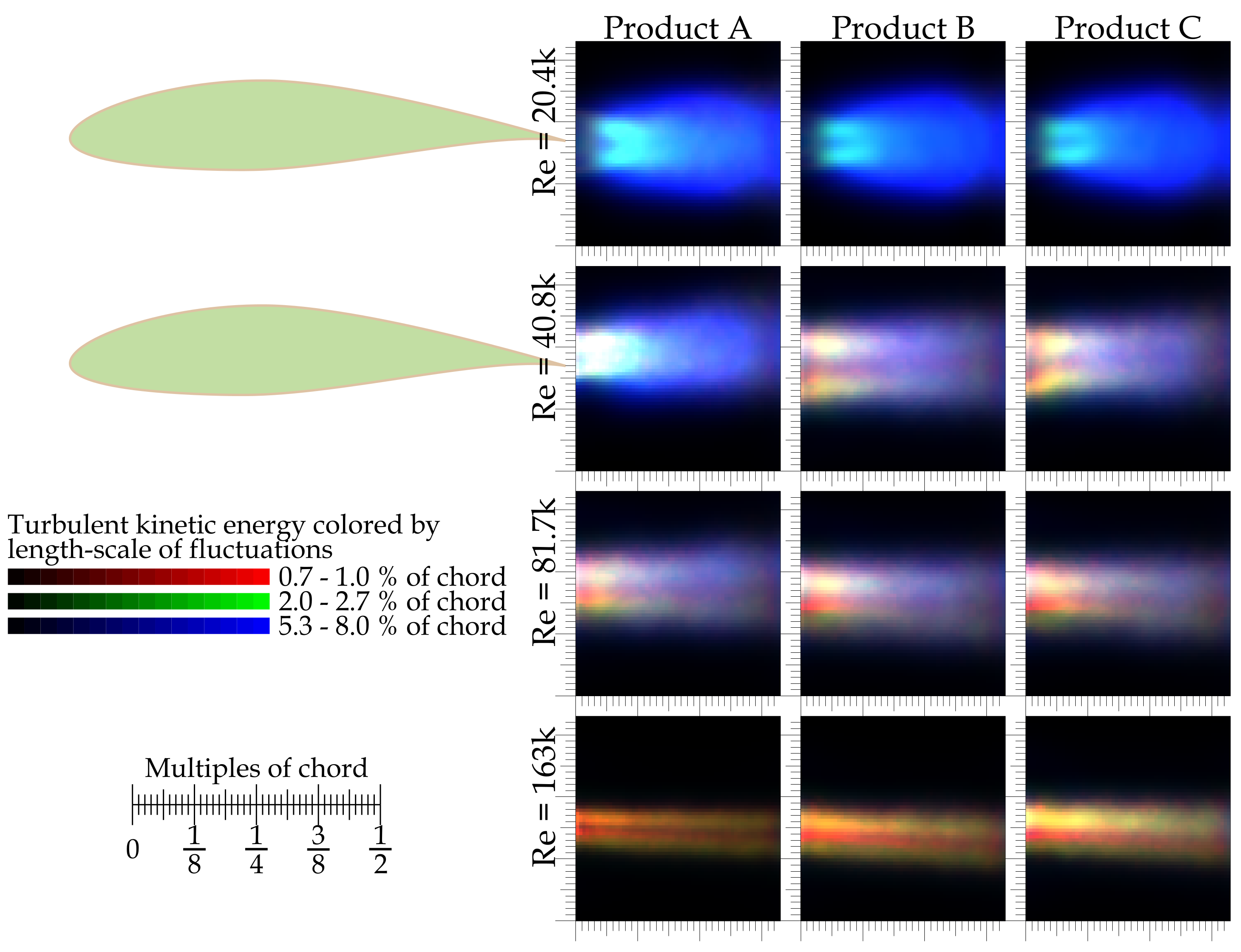
Then, the spatial distribution of turbulent kinetic energies of different bands is calculated. Figure 14 displays the combination of spatial distributions of TKE of three bands depicted by three basic colors: red for the TKE of the spatially smallest fluctuations of length interval 1.0–1.5 grid points, which corresponds to , c chord width; the green channel shows fluctuations of length interval 3–4 grid points, i.e., ; and the blue colors represent the largest resolved fluctuations of sizes between 8–12 grid points—i.e., . The relative intensities of each color channel have to be normalized according to the band interval . Additionally, they are normalized by the famous Kolmogorov scaling [48] in order to obtiain equal color intensities in the case when the power spectral density follows this scaling;
where the effective wave number of an explored band of fluctuations with a size between and is calculated as
and
By using more bands within the spatial resolution of our data, the spatial power spectral density can be reconstructed. It is important to note that, in respect to the classical spectra obtained from time-resolved point data (e.g., [49,50,51]), our method is limited to the range of field of view to the grid point. This interval covers only values from to ; i.e., one and a half orders of magnitude. The classical time-resolved point measurements typically cover tens of minutes by the resolution of tens of kilohertz covering five orders of magnitude in frequency [52]. Our approach shows the spectra calculated by using the entire field of view; each point is affected by all other points in the data ensemble. Moreover, the signal at larger scales feels larger with neighboring areas, while the smallest scale signal is almost local.
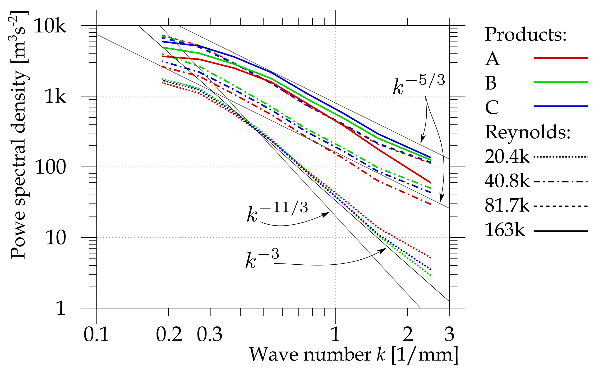
The spatial distribution of length-scale dependent TKE is shown in Figure 14. At lower Re, there are large areas displaying the relative large-scale source of TKE, which is displayed as a massive blue spot. This is caused by large almost laminar vortices in the forming von Kármán vortex street. At Re , the wake past the product A belongs rather to the previous regime, while the others belong to the next regime, characterized by continuing boundary layers containing small scale fluctuations. The wake is still affected by larger scale oscillations of the wake; thus, it is displayed in violet colors—it contains large scales and small scales, while the middle scales are depleted. At even higher Re, the importance of large scales decreases, and the asymmetry appears between the pressure and suction side of the wake—there are more middle-scale fluctuations (green) past the pressure side. At the highest explored Re , the large scales are weaker, and the wake consists of a pair of strips of middle and small-scale fluctuations (yellow) with a strip of small scales (red) in between. We mention again that the dominance of some color in Figure 14 signifies that there is slightly more energy in the corresponding length-scale-band than would be in the case of ideal turbulence following the five-thirds law. Therefore, the energy content of large-scale fluctuations at the highest Reynolds number is still larger than the two other bands combined in absolute numbers. This issue is more apparent in the plot of the power spectral density in Figure 16.
The power spectral density, shown in Figure 16, displays scaling at the smallest Re. We mention that even steeper scaling is typical for a two-dimensional arrangement of vortices [53], which is typically observed in the low Reynolds number wake past the circular cylinder. At higher Reynolds numbers, the spectra approach the law. Note that the vertical axis is not normalized by ; it displays absolute numbers. Despite this, the wake at Re displays less large-scale energy than the wake at Re , while at middle and small-scale wave numbers, the larger Re contains more energy.
3.7. Spatial Correlation
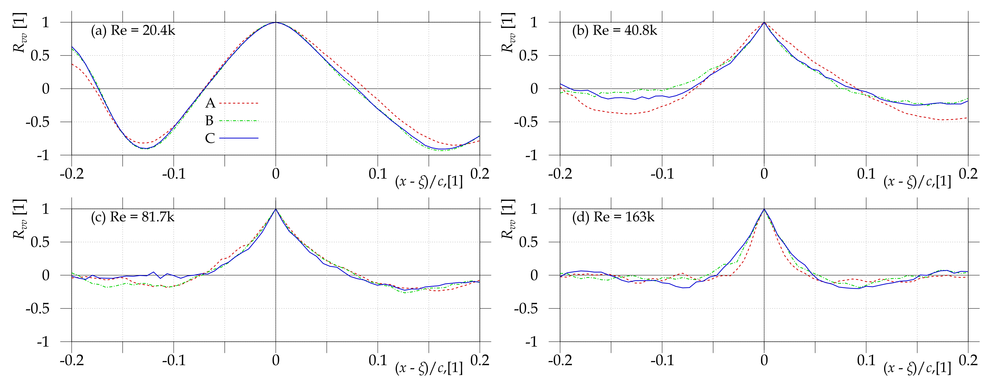
Another way of exploring the size of turbulent structures is the usage of the autocorrelation functions or the structure functions [54,55]. Here, the autocorrelation function of the cross-stream velocity component is used, because this component is active in the formation of the von Kármán vortex street observed at the lower Reynolds numbers. The autocorrelation of some quantity between two separate points and is defined as
where signifies the ensemble averaging and is the standard deviation; is a fluctuation velocity, . In Figure 17, the position vector runs over the entire FoV, while the reference point is fixed in the FoV center.
One of the natural properties of the correlation function is that it inherits some aspects of the basic function; e.g., its periodicity. Therefore, the periodic von Kármán vortex street is reflected as a periodic function of autocorrelation with minima in the distance of half of the spatial period. Note that the distance of the minimum is shorter in the upstream direction and longer in the downstream direction (e.g., at Re , Figure 18a, the minimum in the upstream direction occurs at a. distance of for the case A and at for B and C, while in the upstream direction, the first minimum is for A and for B and C). With increasing Re, the dominant periodic behavior disappears, and the starts to represent the spatial decay of coherence.
The level of spatial coherence is characterized by the integral length-scale, which is defined as the integral of up to some distance M, where reaches zero,
However, reaching zero is not straightforward, as all experimental data contain noise. Thus, the autocorrelation oscillates around zero; see Figure 18, later panels. Azevedo et al. [56] explore several possibilities of the limits of this integral. Here, the simplest key is chosen: the integration is stopped at the distance where reaches the value . This choice underestimates the integral length-scale, as shown in [56], but it does this in a most systematic way.
The values of integral length-scales integrated up to the distance where are plotted in Figure 19. Panel (a) of Figure 19 shows along the stream-wise direction in millimeters. decays systematically and continuously with increasing Re. Note that the interpretation of depends on the regime: at the periodic regime, where is a periodic function with the period of Strouhal shedding, it might represent only a constant fraction of the spatial Strouhal period (suppose that , where a is times the spatial Strouhal frequency, then , where , thus . Rewrite ; then, . ). At the regime dominated by continuing boundary layers, might represent the statistical size of coherent structures, which is the original motivation for this quantity. However, a systematic shortening of is observed without some evidence of regime change. However, if is calculated along the cross-stream direction (panel (c) in Figure 19), the switch of regimes is evident. At lower Reynolds numbers, the observed in the cross-stream direction is as large as the measured area. When the large von Kárm’an street disappears, the value of in the cross-stream direction converges to the range observed in the stream-wise direction (panel (a) of Figure 19). The loss of the large-scale vertical correlation appears at the already discussed regime change at .
The autocorrelation function is not symmetric for upstream and downstream directions, as shown in panel (b) of Figure 19. The asymmetry reaches the value of in favor of the downstream direction. This effect is caused by the increasing average velocity along the stream as the wake widens.
4. Conclusions
We aimed to discover how manufacturing inaccuracies affect the flow topology. The wake behind a single prismatic airfoil NACA 64(3)-618 has been studied experimentally by using the Particle Image Velocimetry (PIV) method. The airfoil has been realized in three copies with a different similarity to the ideal model. The real geometry has been measured by using the 3D optical scanner GOM Atos. We focused on the zero angle of attack at chord-based Reynolds numbers ranging from to .
Generally speaking, the effect of model quality is weaker than the effect of the Reynolds number—the average flow pattern differs more among different velocities than among different models. The deviations in model shape shift the transition between turbulent regimes, which is most observable at a Reynolds number of , where the variant denoted A displays the same regime as for smaller velocities, while the other two realizations B and C produce wakes similar to those observable at higher velocities. This regime change is apparent in the average flow topology (Figure 5), in the decrease of average velocity deficit (Figure 12), in the spatial distribution of the turbulent kinetic energy (Figure 13), in the analysis of isotropy (Figure 6), or in the length-scale of structures producing TKE (Figure 14). This issue can be important if the flow machine (e.g., wind turbine) was designed to operate at the edge of some regime.
The worst variant A differs from the ideal geometry mainly in the quality of trailing edge: it is shorter by ( of the chord length), and it lacks the entire small trail pointing to the pressure side of the airfoil; see Figure 1. Thus, it produces the smallest lift (Figure 9), but also the smallest drag (Figure 20), as the other variants are slightly expanded by using the Minkowski sum. Despite this huge discrepancy, the flow characteristics of this realization are comparable to the better models. The wake centerline orientation is similar to others (Figure 10), the wake thickness reaches similar values (Figure 12), and even the length-scales of fluctuations in the wake display similar patterns (Figure 14) and spectra (Figure 16) as the better versions.
In future, we plan to compare these results with a numerical simulation covering not only the scanned geometry but also the ideal design, which was not accessible by this experiment.
Author Contributions
Conceptualization, D.D. and V.U.; methodology, V.U.; software, D.D.; validation, V.T., V.Y. and V.U.; formal analysis, D.D.; investigation, D.D.; resources, V.U.; data curation, D.D.; writing—original draft preparation, D.D.; writing—review and editing, V.Y. and V.U.; visualization, D.D.; supervision, V.U.; project administration, V.U.; funding acquisition, V.U. All authors have read and agreed to the published version of the manuscript.
Funding
The work was supported by the ERDF under project “Research Cooperation for Higher Efficiency and Reliability of Blade Machines (LoStr)” No. CZ.02.1.01/0.0/0.0/16_026/0008389. The article processing fee has been paid by the European Union, as part of the project entitled “Development of capacities and environment for boosting the international, intersectoral and interdisciplinary cooperation at UWB”, project reg. No. CZ.02.2.69/0.0/0.0/18_054/0014627.
Institutional Review Board Statement
Not applicable.
Informed Consent Statement
Not applicable.
Data Availability Statement
The measured PIV data are available in uloz.to (5.2 GB, accessed on 20 July 2022).
Acknowledgments
We thank Jaroslav Synáč for a discussion about geometry modifications, Petr Eret for maintaining the project, and Jan Narovec for help during the PIV measurement. We thank to Tetjana Tomášková for help with fee payment. The work was supported by the ERDF under project “Research Cooperation for Higher Efficiency and Reliability of Blade Machines (LoStr)” No. CZ.02.1.01/0.0/0.0/16_026/0008389. The article processing fee has been paid by the European Union, as part of the project entitled “Development of capacities and environment for boosting the international, intersectoral and interdisciplinary cooperation at UWB”, project reg. No. CZ.02.2.69/0.0/0.0/18_054/0014627.
Conflicts of Interest
The authors declare no conflict of interest.
Appendix A. Large Angle of Attack
Increasing the angle of attack can, generally, increase the lift coefficient even at symmetrical airfoils. However, it works only up to a critical angle, where a stall occurs. In this study, we measured only angles and , which is quite a large angle. The separation bubble is well resolvable in the plots of the ensemble-average stream-wise velocity in Figure A1. The critical velocity of stall has been not measured at certain , and neither have the critical angles of stall been explored at a certain velocity. The only information that can be read from our data is that at , the stall-critical Reynolds number lies between and .
Figure A1.
Map of ensemble average of stream-wise velocity u at angle of attack . In respect to Figure 4, here is an added row denoted (*) containing data at in order to show that the flow is adhered at this velocity.
Figure A1.
Map of ensemble average of stream-wise velocity u at angle of attack . In respect to Figure 4, here is an added row denoted (*) containing data at in order to show that the flow is adhered at this velocity.

Similarly, the wake centerline points towards the pressure side of the airfoil since ; at lower velocities, it points towards the suction side (up in images). The centerline is determined as a set of points, where , which highlights minima as well as maxima of the cross-stream velocity profiles; see Figure A2.
Figure A2.
Lines of extrema of in cross-stream direction . The number in the top-right corner of each panel is the chord-based Reynolds number, and k denotes . Angle of attack in all panels.
Figure A2.
Lines of extrema of in cross-stream direction . The number in the top-right corner of each panel is the chord-based Reynolds number, and k denotes . Angle of attack in all panels.

The difference among airfoil variants is best visible in the plot of TKE in Figure A3. The flow past variant A at a Reynolds number of clearly displays a different regime than the flow past B and C variants. As discussed above, this discrepancy could be caused by the slightly smaller size of A and thus slightly smaller true. Thus, in Figure A3 and Figure A4, one row is plotted in advance, and that row contains data at an even smaller Reynolds number of . The topology of the wake past product A at is more similar to the wake past all variants at . However, the plot of the length-scale-dependent TKE (Figure A4) reveals the difference between A and B and C even at the smallest explored Reynolds number—wakes past all products are dominated by the largest length-scale at this Re, but the products B and C contain a slightly larger amount of middle-scales and the maxima are better separated than past the A variant.
Figure A3.
Map of turbulent kinetic energy at angle of attack . The first row is added; it is denoted (*) and contains data at in order to show that the wake past product A at belongs to the previous regime.
Figure A3.
Map of turbulent kinetic energy at angle of attack . The first row is added; it is denoted (*) and contains data at in order to show that the wake past product A at belongs to the previous regime.

Figure A4.
Turbulent kinetic energy colored by the length-scale of fluctuations producing it. TKE is divided into three channels: the red channel represents the smallest length-scale of fluctuations, the green channel shows fluctuations of middle sizes, and the blue represents the largest fluctuations. The color scale for different color channels is normalized in such a way that an ideal Kolmogorov turbulence would be displayed in shades of gray. Among different Re and variants, the color scale is automatically adapted (for differences in amounts of TKE, look to Figure A3. Rows denoted by (*) are added.

At between and , the wake contains small-scale fluctuations in its pressure side (bottom part of figures), while in the suction side (upper in figures), it contains mostly fluctuations of larger scales that are depleted by small scales, because the shear layer turbulence is older here (the flow is detached close to the leading edge; then, it develops, dissipating energy at the smallest scales due to the viscosity. Therefore, the smallest scales are depleted first). Thus, the upper shear layer in Figure A4 is less localized and constructed by fluctuations of larger scales.
At , the flow is attached, as has been discussed above and shown in Figure A1, but the suction side of the wake still contains a significantly stronger signal from large-scale fluctuations, because the boundary layer at the suction side (top) is less stable than at the pressure side (bottom). At an even higher Reynolds number, the boundary layer is more stable, and the wake does not contain a large-scale (blue) signal anymore; however, there is an asymmetry between the pressure and suction sides. The autocorrelation function in Figure A5 shows the same pattern—the coherent structures are significantly larger inside the suction part of the wake than in the pressure part. The different airfoil variants follow more or less the same pattern. Only the variant B displays stronger periodic behavior at in the autocorrelation with a reference point in the pressure part of the wake; see Figure A5b.
Figure A5.
Autocorrelation function of fluctuating cross-stream velocity component v at two Reynolds numbers (a) and (b), where the flow is attached at . First, the autocorrelation with the reference point in the suction part of the wake (top) and second with the reference point in the pressure part of the wake (bottom).

The spatial spectra, whose construction has been shortly described above or in more detail in our previous publication [24], are plotted in Figure A6 for the angle of attack . There, the contrast between the adhered flow at (displayed by solid lines) and the smaller velocities with stall is visible. The largest contains less energy at the largest scales than the flow at four times smaller velocity. At middle scales, it contains a comparable amount of energy to the flow at half the velocity. The power spectral density is steeper than the Kolmogorov scaling, except for the largest k, where the instrumental noise appears. This scaling is even steeper at larger scales (which is not valid for the largest ).
Figure A6.
Spatial spectrum of the turbulent kinetic energy at . Products are distinguished with colors, Reynolds numbers wuith different line styles. The thin black lines represent the scaling.
Figure A6.
Spatial spectrum of the turbulent kinetic energy at . Products are distinguished with colors, Reynolds numbers wuith different line styles. The thin black lines represent the scaling.

References
- Frisch, U.; Kolmogorov, A.N. Turbulence: The legacy of AN Kolmogorov; Cambridge University Press: Cambridge, UK, 1995. [Google Scholar]
- AIAA. Guide for the Verification and Validation of Computational Fluid Dynamics Simulations; G-077; AIAA: Reston, VA, USA, 1998. [Google Scholar] [CrossRef]
- Drela, M. Airfoil Tools. Available online: http://airfoiltools.com. (accessed on 20 April 2021).
- Moreno-Oliva, V.I.; Román-Hernández, E.; Torres-Moreno, E.; Dorrego-Portela, J.R.; Avendaño Alejo, M.; Campos-García, M.; Sánchez-Sánchez, S. Measurement of quality test of aerodynamic profiles in wind turbine blades using laser triangulation technique. Energy Sci. Eng. 2019, 7, 2180–2192. [Google Scholar] [CrossRef] [Green Version]
- Drela, M. XFOIL: An Analysis and Design System for Low Reynolds Number Airfoils. In Proceedings of the Low Reynolds Number Aerodynamics, Notre Dame, IA, USA, 5–7 June 1989; Volume 54, pp. 1–12. [Google Scholar] [CrossRef]
- Ravikovich, Y.; Kholobtsev, D.; Arkhipov, A.; Shakhov, A. Influence of geometric deviations of the fan blade airfoil on aerodynamic and mechanical integrity. J. Phys. Conf. Ser. 2021, 1891, 012042. [Google Scholar] [CrossRef]
- Klimko, M.; Okresa, D. Measurements in the VT 400 air turbine. Acta Polytech. 2016, 56, 118. [Google Scholar] [CrossRef] [Green Version]
- Uher, J.; Milcak, P.; Skach, R.; Fenderl, D.; Zitek, P.; Klimko, M. Experimental and Numerical Evaluation of Losses From Turbine Hub Clearance Flow. Turbo Expo Power Land Sea Air 2019, 2B, 9. [Google Scholar] [CrossRef]
- Winstroth, J.; Seume, J.R. On the influence of airfoil deviations on the aerodynamic performance of wind turbine rotors. J. Phys. Conf. Ser. 2016, 753, 022058. [Google Scholar] [CrossRef] [Green Version]
- Alsoufi, M.S.; Elsayed, A.E. Surface Roughness Quality and Dimensional Accuracy—A Comprehensive Analysis of 100% Infill Printed Parts Fabricated by a Personal/Desktop Cost-Effective FDM 3D Printer. Mater. Sci. Appl. 2018, 09, 11–40. [Google Scholar] [CrossRef] [Green Version]
- Inkinen, S.; Hakkarainen, M.; Albertsson, A.; Södergøard, A. From lactic acid to poly(lactic acid) (PLA): Characterization and analysis of PLA and Its precursors. Biomacromolecules 2011, 12, 523–532. [Google Scholar] [CrossRef]
- Zhang, C.; Zhao, H.; Gu, F.; Ma, Y. Phase unwrapping algorithm based on multi-frequency fringe projection and fringe background for fringe projection profilometry. Meas. Sci. Technol. 2015, 26. [Google Scholar] [CrossRef]
- Li, F.; Stoddart, D.; Zwierzak, I. A Performance Test for a Fringe Projection Scanner in Various Ambient Light Conditions. Procedia CIRP 2017, 62, 400–404. [Google Scholar] [CrossRef]
- GOM. GOM Acceptance Test—Process Description, Acceptance Test according to the Guideline VDI/VDE 2634 Part 3; Engl. VDI/VDE-Gesellschaft Mess- und Automatisierungstechnik: Düsseldorf, Germnay, 2014. [Google Scholar]
- Mendricky, R. Determination of measurement accuracy of optical 3D scanners. MM Sci. J. 2016, 2016, 1565–1572. [Google Scholar] [CrossRef] [Green Version]
- Vagovský, J.; Buranský, I.; Görög, A. Evaluation of measuring capability of the optical 3D scanner. Procedia Eng. 2015, 100, 1198–1206. [Google Scholar] [CrossRef] [Green Version]
- Du, W.; Zhao, Y.; He, Y.; Liu, Y. Design, analysis and test of a model turbine blade for a wave basin test of floating wind turbines. Renew. Energy 2016, 97, 414–421. [Google Scholar] [CrossRef]
- GOM. ATOS Core. Available online: https://www.gom.com/en/products/3d-scanning/atos-core (accessed on 20 April 2021).
- Krein, M.; Šmulian, V. On Regularly Convex Sets in the Space Conjugate to a Banach Space. Ann. Math. 1940, 41, 556–583. [Google Scholar] [CrossRef]
- Yanovych, V.; Duda, D.; horáček, V.; Uruba, V. Research of a wind tunnel parameters by means of cross-section analysis of air flow profiles. AIP Conf. Proc. 2019, 2189. [Google Scholar] [CrossRef]
- Yanovych, V.; Duda, D. Structural deformation of a running wind tunnel measured by optical scanning. Stroj. Cas. 2020, 70, 181–196. [Google Scholar] [CrossRef]
- Duda, D.; Yanovych, V.; Uruba, V. An experimental study of turbulent mixing in channel flow past a grid. Processes 2020, 8, 1355. [Google Scholar] [CrossRef]
- Tropea, C.; Yarin, A.; Foss, J.F. Springer Handbook of Experimental Fluid Mechanics; Springer: Berlin/Heidelberg, Germany, 2007; p. 1557. [Google Scholar]
- Duda, D.; Uruba, V. Spatial Spectrum From Particle Image Velocimetry Data. ASME J. Nucl. Rad. Sci. 2019, 5, 030912. [Google Scholar] [CrossRef]
- Von Kármán, T. Aerodynamics. In McGraw-Hill Paperbacks: Science, Mathematics and Engineering; McGraw-Hill: New York, NY, USA, 1963. [Google Scholar]
- Drela, M. Low-Reynolds Number Airfoil Design for the MIT Daedalus Prototype: A Case Study. J. Aircr. 1988, 25, 724–732. [Google Scholar] [CrossRef]
- Drela, M.; Giles, M. Viscous-Inviscid Analysis of Transonic and Low Reynolds Number Airfoils. AIAA J. 1987, 25, 1347–1355. [Google Scholar] [CrossRef]
- Terra, W.; Sciacchitano, A.; Scarano, F. Aerodynamic drag of a transiting sphere by large-scale tomographic-PIV. Exp. Fluids 2017, 58. [Google Scholar] [CrossRef] [Green Version]
- Terra, W.; Sciacchitano, A.; Scarano, F. Drag analysis from PIV data in speed sports. Procedia Eng. 2016, 147, 50–55. [Google Scholar] [CrossRef] [Green Version]
- Ragni, D.; Oudheusden, B.W.; Scarano, F. Non-intrusive aerodynamic loads analysis of an aircraft propeller blade. Exp. Fluids 2011, 51, 361–371. [Google Scholar] [CrossRef] [Green Version]
- Oudheusden, B.W. PIV-based pressure measurement. Meas. Sci. Technol. 2013, 24, 032001. [Google Scholar] [CrossRef]
- Antonia, R.A.; Rajagopalan, S. Determination of drag of a circular cylinder. AIAA J. 1990, 28, 1833–1834. [Google Scholar] [CrossRef]
- Zhou, Y.; Alam, M.M.; Yang, H.; Guo, H.; Wood, D. Fluid forces on a very low Reynolds number airfoil and their prediction. Int. J. Heat Fluid Flow 2011, 32, 329–339. [Google Scholar] [CrossRef] [Green Version]
- Mohebi, M.; Wood, D.H.; Martinuzzi, R.J. The turbulence structure of the wake of a thin flat plate at post-stall angles of attack. Exp. Fluids 2017, 58. [Google Scholar] [CrossRef]
- Duda, D.; Yanovych, V.; Uruba, V. Wake Width: Discussion of Several Methods How to Estimate It by Using Measured Experimental Data. Energies 2021, 14, 4712. [Google Scholar] [CrossRef]
- Eames, I.; Jonsson, C.; Johnson, P.B. The growth of a cylinder wake in turbulent flow. J. Turbul. 2011, 12, N39. [Google Scholar] [CrossRef]
- Romano, G.P. Large and small scales in a turbulent orifice round jet: Reynolds number effects and departures from isotropy. Int. J. Heat Fluid Flow 2020, 83. [Google Scholar] [CrossRef]
- Lumley, J.L.; Newman, G. The return to isotropy of homogeneous turbulence. J. Fluid Meach. 1977, 82, 161–178. [Google Scholar] [CrossRef] [Green Version]
- Simonsen, A.J.; Krogstad, P.o. Turbulent stress invariant analysis: Clarification of existing terminology. Phys. Fluids 2005, 17, 088103. [Google Scholar] [CrossRef] [Green Version]
- Choi, K.; Lumley, J.L. The return to isotropy of homogeneous turbulence. J. Fluid Meach. 2001, 436, 59–84. [Google Scholar] [CrossRef]
- Duda, D.; Bém, J.; Yanovych, V.; Pavlíček, P.; Uruba, V. Secondary flow of second kind in a short channel observed by PIV. Eur. J. Mech. B/Fluids 2020, 79, 444–453. [Google Scholar] [CrossRef]
- Bém, J.; Duda, D.; Kovařík, J.; Yanovych, V.; Uruba, V. Visualization of secondary flow in a corner of a channel. AIP Conf. Proc. 2019, 2189, 020003-1-6. [Google Scholar] [CrossRef]
- Kundu, P.; Cohen, I.; Dowling, D. Fluid Mechanics, 6th ed.; Academic Press: Cambridge, MA, USA, 2016. [Google Scholar]
- Duda, D.; Uruba, V. PIV of air flow over a step and discussion of fluctuation decompositions. AIP Conf. Proc. 2018, 2000, 020005. [Google Scholar] [CrossRef]
- Agrawal, A. Measurement of spectrum with particle image velocimetry. Exp. Fluids 2005, 39, 836–840. [Google Scholar] [CrossRef]
- Agrawal, A.; Prasad, A. Properties of vortices in the self-similar turbulent jet. Exp. Fluids 2002, 33, 565–577. [Google Scholar] [CrossRef]
- Duda, D.; La Mantia, M.; Skrbek, L. Streaming flow due to a quartz tuning fork oscillating in normal and superfluid He 4. Phys. Rev. B 2017, 96. [Google Scholar] [CrossRef]
- Kolmogorov, A.N. Dissipation of Energy in the Locally Isotropic Turbulence. Proc. R. Soc. A Math. Phys. Eng. Sci. 1991, 434, 15–17. [Google Scholar] [CrossRef]
- Jiang, M.T.; Law, A.W.K.; Lai, A.C.H. Turbulence characteristics of 45 inclined dense jets. Environ. Fluid Mech. 2018, 1–28. [Google Scholar] [CrossRef]
- Barenghi, C.F.; Sergeev, Y.A.; Baggaley, A.W. Regimes of turbulence without an energy cascade. Sci. Rep. 2016, 6, 1–11. [Google Scholar] [CrossRef] [PubMed] [Green Version]
- Harun, Z.; Abbas, A.A.; Lotfy, E.R.; Khashehchi, M. Turbulent structure effects due to ordered surface roughness. Alex. Eng. J. 2020, 59, 4301–4314. [Google Scholar] [CrossRef]
- Bourgoin, M.; Baudet, C.; Kharche, S.; Mordant, N.; Vandenberghe, T.; Sumbekova, S.; Stelzenmuller, N.; Aliseda, A.; Gibert, M.; Roche, P.; et al. Investigation of the small-scale statistics of turbulence in the Modane S1MA wind tunnel. CEAS Aeronaut. J. 2018, 9, 269–281. [Google Scholar] [CrossRef]
- Kraichnan, R.H. Inertial ranges in two-dimensional turbulence. Phys. Fluids 1967, 10, 1417–1423. [Google Scholar] [CrossRef] [Green Version]
- Schulz-DuBois, E.O.; Rehberg, I. Structure Function in Lieu of Correlation Function. Appl. Phys. 1981, 24, 323–329. [Google Scholar] [CrossRef]
- Kubíková, T. The air flow around a milling cutter investigated experimentally by particle image velocimetry. AIP Conf. Proc. 2021, 2323, 030006-1-8. [Google Scholar] [CrossRef]
- Azevedo, R.; Roja-Solórzano, L.R.; Bento Leal, J. Turbulent structures, integral length scale and turbulent kinetic energy (TKE) dissipation rate in compound channel flow. Flow Meas. Instrum. 2017, 57, 10–19. [Google Scholar] [CrossRef]
Figure 1.
(a) Comparison of 3D scans of three manufactured realizations of the NACA 64-618 airfoil, which is depicted by a solid black line. The production details are in text. Panels (b) and (c) show the enlarged details of the leading and trailing edge, respectively.
Figure 1.
(a) Comparison of 3D scans of three manufactured realizations of the NACA 64-618 airfoil, which is depicted by a solid black line. The production details are in text. Panels (b) and (c) show the enlarged details of the leading and trailing edge, respectively.

Figure 2.
(a) Position of the area studied by using Particle Image Velocimetry, depicted as a blue square just behind the trailing edge of the airfoil. The PIV area is a square of side . The estimated thickness of the illuminated plane is . The laser light comes from the counter-stream direction. (b–d) Photograph of the 3D printed realizations of the airfoil. Their trailing parts are blacked in order to suppress the laser reflections.

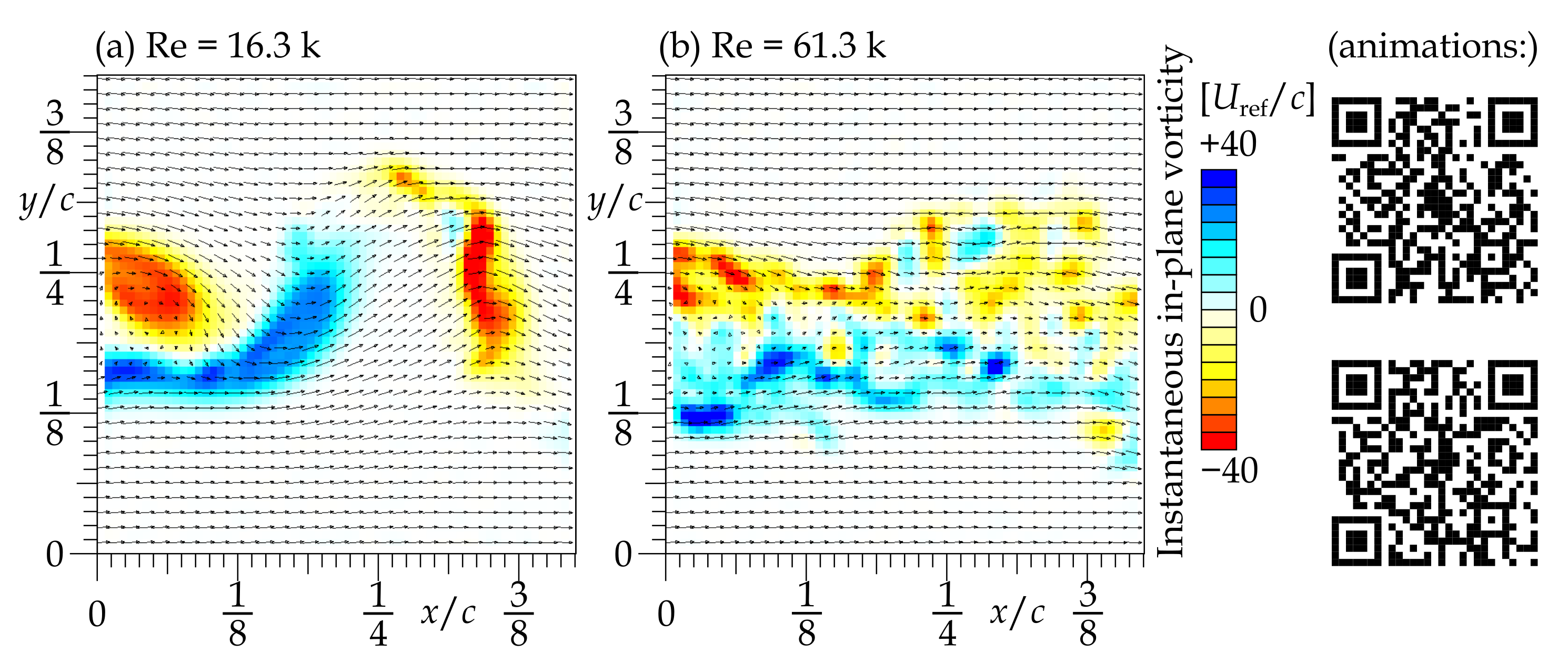
Figure 3.
The example of instantaneous velocity fields at chord-based Reynolds numbers (a) and (b), both at zero angle of attack. Only every second velocity vector is displayed. The color in the background represents the z-component of vorticity . The QR codes link to http://home.zcu.cz/~dudad/PIV_uplav_3ms.gif and http://home.zcu.cz/~dudad/PIV_uplav_12ms.gif (accessed on 20 July 2021) show the pair of photos used to draw this figure.

Figure 4.
First three columns show the map of average stream-wise velocity u normalized by the reference velocity past the slightly different samples A, B, and C. The fourth column displays isotachs together. The green tips on the left edge of the figure represent the positions of the airfoil trailing edge. The Reynolds number is based on the chord length and the reference velocity. The reference velocity is measured in the empty wind tunnel under otherwise similar conditions. Angle of attack in all panels.

Figure 5.
The cross-stream profile of average stream-wise velocity at stream-wise distance past the trailing edge. Angle of attack in all panels. The uncertainty is displayed via the area.
Figure 5.
The cross-stream profile of average stream-wise velocity at stream-wise distance past the trailing edge. Angle of attack in all panels. The uncertainty is displayed via the area.

Figure 6.
The ratio of cross-stream fluctuations to stream-wise fluctuations obtained behind three different manufactured samples, denoted A, B, and C. Angle of attack in all panels. Redder colors signify a dominance of stream-wise fluctuations, which is typical for areas of continuing boundary layer, while the bluer colors highlight areas of stronger cross-stream fluctuations, which is typical for the so-called true wake.

Figure 7.
The cross-stream profile of average cross-stream velocity at stream-wise distance past the trailing edge. Angle of attack in all panels.
Figure 7.
The cross-stream profile of average cross-stream velocity at stream-wise distance past the trailing edge. Angle of attack in all panels.

Figure 8.
Sketch and photograph of the balance used for lift force measurement. The metallic flexible elements are connected to the wind tunnel walls at their upper end. The airfoil is reinforced by using an aluminum tube, which connects the airfoil to the movable table as well. The eddy-current sensor is used to electrically measure the displacement of the entire table.

Figure 9.
Balance measurement of the lift coefficient. The theoretical results for ideal geometry are displayed as well. Angle of attack .
Figure 9.
Balance measurement of the lift coefficient. The theoretical results for ideal geometry are displayed as well. Angle of attack .

Figure 10.
(a–d) Lines of extrema of along cross-stream direction . The number in the top-right corner of each panel is the chord-based Reynolds number, and k denotes . (e) Direction of centerline as a function of the Reynolds number. It is obtained as a linear fit of the coordinates of the minima of transverse profiles. Angle of attack in all panels.

Figure 11.
Solid lines indicate the wake width as a function of distance past the airfoil trailing edge, x; the corresponding axis is on the left-hand-side of the plots. Dashed lines represent the maximum deficit velocity as a function of x; the axes for these values are on the right-hand-side of the plots. Different panels contain data at different Reynolds numbers and angle of attack .

Figure 12.
(Top left) Dependence of the wake width at a fixed stream-wise distance past the trailing edge on the chord-based Reynolds number. (Top right) Dependence of the velocity deficit at a certain distance on the Reynolds number. (Bottom left) Dependence of the growth rate of the wake width a on the Reynolds number. (Bottom right) Decay rate of velocity deficit, if a hyperbolic decrease is expected. Angle of attack in all panels.

Figure 13.
Turbulent kinetic energy (TKE) based on in-plane velocities only (thus, it is thought to be underestimated) obtained behind three different manufactured samples denoted A, B, and C. The scale is adapted to except for the last line, where the scale is . Angle of attack in all panels.
Figure 13.
Turbulent kinetic energy (TKE) based on in-plane velocities only (thus, it is thought to be underestimated) obtained behind three different manufactured samples denoted A, B, and C. The scale is adapted to except for the last line, where the scale is . Angle of attack in all panels.

Figure 14.
Turbulent kinetic energy colored by the length-scale of fluctuations producing it at angle of attack . TKE is divided into three channels: the red channel represents fluctuations of sizes 0.7–1.0% of chord width; the green channel shows fluctuations of sizes between 2.0% and 2.7% of chord width; while the blue represents the largest fluctuations of sizes 5.3–8.0% of chord width. The color scale for different color channels is normalized in such a way that an ideal Kolmogorov turbulence would be displayed in shades of gray. Among different Re and variants, the color scale is automatically adapted (for differences in amount of TKE, look to Figure 13 or Figure 15).

Figure 15.
The cross-stream profile of the turbulent kinetic energy (TKE) at stream-wise distance past the trailing edge. Angle of attack in all panels. Note the logarithmic scale.
Figure 15.
The cross-stream profile of the turbulent kinetic energy (TKE) at stream-wise distance past the trailing edge. Angle of attack in all panels. Note the logarithmic scale.

Figure 16.
Spatial spectra of turbulent kinetic energy. The different products are distinguished by color, the Reynolds number by the line style; the angle of attack is zero in all cases. Thin lines represent scalings , , and .
Figure 16.
Spatial spectra of turbulent kinetic energy. The different products are distinguished by color, the Reynolds number by the line style; the angle of attack is zero in all cases. Thin lines represent scalings , , and .

Figure 17.
Autocorrelation function of cross-stream velocity component v with a reference point in the middle of the field of view; i.e., past the trailing edge at .
Figure 17.
Autocorrelation function of cross-stream velocity component v with a reference point in the middle of the field of view; i.e., past the trailing edge at .

Figure 18.
The stream-wise profile of the autocorrelation function of the cross-stream velocity component at .
Figure 18.
The stream-wise profile of the autocorrelation function of the cross-stream velocity component at .

Figure 19.
Integral length-scale of cross-stream velocity component v. Panel (a) shows the integral length-scale along the stream-wise axis; however, it is different in upstream and downstream directions, and panel (b) shows this asymmetry. Panel (c) shows the integral length-scale of v along the cross-stream axis. Angle of attack in all panels.

Figure 20.
Rough estimation of the drag coefficient based only on the momentum deficit and stress term; the pressure term is ignored. Panel (a) is processed via the methodology of Terra et al. [28], while panel (b) shows the drag coefficient estimated according to Antonia and Rajagopalan [32] based on the same PIV data. Black points denote data obtained from the public database Airfoiltools [3] calculated by using the Xfoil [5,26,27] for the . Angle of attack in both panels.


Table 1.
Dimensions of the studied airfoil realizations compared with the ideal case, denoted CAD in the first column. The blockage ratio of the wind tunnel is the ratio of the blocked projection area to the total cross-section area (); it is calculated with the caliper approach—i.e., the distance of the plane touching the suction side to the second plane touching the pressure side, when their normals are locked to the y-axis.
| Unit | CAD | A | B | C | |
|---|---|---|---|---|---|
| Chord length c | mm | ||||
| Profile thickness—maximum inscribed circle | mm | ||||
| Profile thickness—caliper along y-axis | mm | ||||
| Blockage ratio | % |
Publisher’s Note: MDPI stays neutral with regard to jurisdictional claims in published maps and institutional affiliations. |
© 2022 by the authors. Licensee MDPI, Basel, Switzerland. This article is an open access article distributed under the terms and conditions of the Creative Commons Attribution (CC BY) license (https://creativecommons.org/licenses/by/4.0/).
Share and Cite
MDPI and ACS Style
Duda, D.; Yanovych, V.; Tsymbalyuk, V.; Uruba, V. Effect of Manufacturing Inaccuracies on the Wake Past Asymmetric Airfoil by PIV. Energies 2022, 15, 1227. https://doi.org/10.3390/en15031227
AMA Style
Duda D, Yanovych V, Tsymbalyuk V, Uruba V. Effect of Manufacturing Inaccuracies on the Wake Past Asymmetric Airfoil by PIV. Energies. 2022; 15(3):1227. https://doi.org/10.3390/en15031227
Chicago/Turabian StyleDuda, Daniel, Vitalii Yanovych, Volodymyr Tsymbalyuk, and Václav Uruba. 2022. "Effect of Manufacturing Inaccuracies on the Wake Past Asymmetric Airfoil by PIV" Energies 15, no. 3: 1227. https://doi.org/10.3390/en15031227
Note that from the first issue of 2016, this journal uses article numbers instead of page numbers. See further details here.