The Impact of Airport Proximity on Single-Family House Prices—Evidence from Poland


1
Department of Spatial Analysis and Real Estate Market, University of Warmia and Mazury in Olsztyn, Prawocheńskiego 15, 10-720 Olsztyn, Poland
2
Department of Real Estate and Investment Economics, Cracow University of Economics, ul. Rakowicka 27, 31-510 Kraków, Poland
*
Author to whom correspondence should be addressed.
Sustainability 2020, 12(19), 7928; https://doi.org/10.3390/su12197928
Submission received: 24 July 2020
/
Revised: 4 September 2020
/
Accepted: 9 September 2020
/
Published: 24 September 2020
(This article belongs to the Special Issue The Quality of Urban Areas: New Measuring Tools and Methods, Impact on Quality of Life and Costs of Bad Design)
Abstract
:Airports in Poland are obliged to observe the sustainable development principle and therefore to reduce their environmental impact by creating so-called limited use areas (LUA) related to aircraft-generated noise. The research authors analyzed airports’ impact on the prices of single-family homes located in the vicinity of airports. The LUA is therefore defined as the area designated to study the airport’s specific impact on the single-family housing market. This is a formal limit which determines the examination of price changes and the decision-making conditions of market participants. This methodical approach is justified because no excessive noise is expected outside the LUA. Therefore, two markets in the vicinity of airports were examined. One is in an LUA which is closer to the airport, and the other market is outside the LUA where external noise effects are not present. Thus, we consider that real estate located outside the LUA is not subject to a significant negative impact from the airport. The study covered the Gdańsk Lech Walesa Airport and the Warsaw Chopin Airport in Poland in adjacent areas with the research time horizon of 2013–2017. The study examined single-family house prices. We used a time series analysis, a classic multiple regression model, a spatial autoregressive model, and geographically weighted regression models in our research. Additionally, Geographical Information System (GIS) tools were used to visualize the results of our study. The research result was to demonstrate different impact levels of airports on the prices of single-family houses located in limited-use areas in Gdańsk and Warsaw. This research carries significant implications for the general public and airports’ economic decisions in resolving conflicts between the airport and residential property owners in airports’ vicinities.
1. Introduction
The sustainable development concept stipulates that today’s generations’ needs are met without compromising the ability of future generations to meet their own needs in order to ensure intra-generational and intergenerational justice [1,2]. Thus, cities and regions’ sustainable development requires a careful balance between the various development dimensions: economic [3,4], social [5,6], and environmental [7,8]. A clear predominance of one of these three dimensions in the development path would not be characterized as sustainable development. The economic development level has usually been considered as cities’ or regions’ basic development measure, and as a result, the social and environmental dimensions have been neglected or considered to a negligible extent. Profit or value creation have been development’s ultimate purpose, which has resulted in environmental degradation and the perception of a significant part of society only as a mere production factor. In terms of neoclassical economics, market behaviors which lead to resource allocation are most often described with the market equilibrium models which take into account three elements: demand, supply, and price. The economic component’s domination over the social and environmental components disregards the importance of the institutional environment or the market behavioral aspects. The sustainable development concept makes it possible to change the neo-liberal paradigm which has been predominant in economic milieus. The paradigm is based on the rationality–greed–balance triad. Man represents the social dimension in the sustainable development model presented above. In the neo-liberal development paradigm, man is treated as a rational being who acts according to the optimality criterion, i.e., homo oeconomicus (more in [9,10,11,12]). Sustainable development which strives for improvement in economic, social, and ecological dimensions supports other human models [13,14,15,16], including homo reciprocans, neo-homo economicus, or homo socio-economicus. This form of man, or broadly defined society perception, focuses on human behavior strongly conditioned by social, religious, cultural, and gender determinants. The third element of the sustainable development triad is the environmental dimension based on the eco-development concept. According to Górka [17], the eco-development concept refers to socio-economic development related to environment protection and respect for nature. Such a definition does not therefore represent the part of society’s radical-extremist, ecological attitudes including zero-growth theory (more in [18,19]), which postulates the dominance of pro-ecological thinking over the previously quoted economic and social dimensions. Sustainable development in the ecological aspect is therefore an environment protection process [20] through the economic processes of greening [21] in the form of new economic development methods, [22] new technologies [23], and new energy carriers [24], as well as new forms of societal non-economic activity [25], while minimizing the economic development growth-rate slowdown.
The sustainable development concept considered in relation to air traffic and airports’ spatial distribution in urban areas requires a multi-layered and multi-dimensional approach. Air transport contributes to the economic development of cities and regions by stimulating production and employment in other sectors [26]. Airports are becoming nodes of the international and national economic system: they are powerful agents of local economic development, attracting passenger traffic and service activities directly, and are indirectly linked to the airport system (hotels, retail trade, centers of entertainment, commercial and exhibition complexes, office buildings, warehouses, and distribution services) [27]. The fast transport of people and commodities via airports includes airport cities or regions in global economic processes. An airport can even be compared to an infrastructural gate towards the global bloodstream which circulates export and import products for enterprises. The network connection positive effect includes [28,29] increasing enterprises’ income, tourist traffic, and new investments, and, as a result, causes the unemployment rate to decrease.
Air traffic’s undeniable positive impact on cities’ and regions’ development is offset, to some extent, by several negative effects. An airport located in an urban zone or absorbed by the city’s sprawl results in airport neighborhood-related nuisance and the inability to meet noise and air quality environmental standards. This refers to the sustainable development triad presented earlier (economy–environment–society). The environmental aspect is mainly represented by aircraft-emitted noise (during landing and take-off operations), however, the co-existing air pollution has gained significance. These factors’ negative impact level is closely correlated with airport size and air traffic intensity. In the case of very large airports located in different parts of the world (e.g., Hartsfield–Jackson Atlanta International Airport, Los Angeles International Airport, London Heathrow, or İstanbul Atatürk Airport), negative health effects were observed among inhabitants in the closest airport vicinity [30,31], including lung and heart diseases, distraction, hyperactivity, and fatigue.
Airports’ and air traffic’s positive impact (economic aspect) coupled with their negative impact (environmental aspect) affects the third sustainable development aspect (the social one). In Poland, the creation of special zoning around airports is one of the ways to minimize the social and environmental costs generated by airport locations in cities (proximity to residential buildings); these are the so-called limited use areas (LUA). According to Cellmer et al. [32], although the introduction of such an area in the vicinity of an airport may introduce restrictions in the permissible use of land (principles of land development and its uses), it supports the owners in obtaining compensation for these limitations and provides an opportunity to obtain reimbursement of costs spent on acoustic upgrading of their houses. Additionally, in the same article, detailed spatial analyses were carried out concerning the spatial distribution of real estate prices in the vicinity of the airport in Warsaw (Poland). The current article represents the development of our previous [32] with a comparison of time series models and spatial models to the Gdańsk Lech Walesa Airport and Warsaw Chopin Airport in Poland. We also modified the database, standardized the data, introduced new research methods, and presented a much broader context of the problem and its importance for sustainable development. According to Batóg et al. [33], negative airport externalities (noise or pollution) decrease both residential satisfaction in the area affected and property values. Additionally, restrictions on land use (for example, related to residential development), a lower density of development, and additional technical regulations (sound isolation requirements) may have a detrimental effect on property prices. According to Habdas and Konowalczuk [34], the creation of limited use areas in Poland is related to the fact that the law allows to exceed the acceptable environmental impact standards within LUAs; thus, owners of property within LUAs may be subject to restrictions on the property development and use for specific purposes. Therefore, limited use area zoning may (although not necessarily) entail restrictions on how a property is used. Because of the multidimensional and interdisciplinary research subject, this article focuses on the sustainable development’s social aspect in the context of satisfying basic human needs, i.e., housing needs. Through housing price changes, the housing market responds to both its positive and negative environment changes.
This article examines the airport negative impact on single-family houses prices located in the vicinity of airports. In our research, this spatial impact extent on real estate is determined with the limited use area (LUA) boundaries created around a given airport, because no excessive noise is recorded outside the LUA. Thus, properties located outside the LUA are considered outside significant negative airports’ impact. The research examines the impact on the prices of single-family houses of the two airports in Poland—Warsaw and Gdańsk. The limited use areas for Gdańsk Lech Walesa Airport and Warsaw Chopin Airport concerning single-family houses do not impose building or extension restrictions. These areas’ inhabitants acquire the right to compensate for airport arduousness related to actual or foretasted noise levels exceedance; they are offered reimbursement of the actual costs incurred to adapt buildings to acoustic requirements. We used a time series analysis and a classic multiple regression model, a spatial autoregressive model and geographically weighted regression models, in our research. Additionally, Geographical Information System (GIS) tools were used to visualize the results of our study.
The paper is organized as follows. The next section presents a review of the related literature and a brief description of previous studies on the relationships between air traffic, airports, and the housing market. The third chapter presents the study area, data collection, and a description of research methods used. In Section 4, we present the results and discussion with a description of major findings of our empirical investigation, as well as discussing the limitation of the results. The last section presents remarks and conclusions drawn throughout this work.
2. Literature Review
Airborne traffic is one of the most effective forms of passenger and cargo transportation [29,35,36] and thus an important development factor for cities and regions [27,37]. The air traffic development results in new airports creation or the expansion of existing ones. The problem of airports located in the urban zone having an impact on the environment is broadly discussed in the literature on the subject.
Wolfe et al. [38] examined the environmental costs for people living in the vicinity of 84 commercial airports in the United States, with particular emphasis on air quality, noise levels, and climate change impacts. The study investigated how individuals bear the environmental impacts of a year of aviation operations as a function of their distance from an airport. Results have demonstrated that aircraft noise level-related damage dominates at a distance of less than 6 km from airports. At distances greater than 6 km, damages from climate change or air quality damages from cruise emissions dominate environmental costs. Barett et al. [39] show the global effect of aircraft emissions on human health through the degradation of air quality. Levy et al.’s research [40] based on the Community Multiscale Air Quality (CMAQ) model with the Speciated Modelled Attainment Test (SMAT) for 99 US-based airports assessed negative air quality and its impact on the health condition of the general public living in the airport’s vicinity. In another study based on 76 European airports, Mashhoodi and Timmeren [41], based on population density, distribution of urbanized areas, location of agricultural lands, location of the natural area, and distribution of leisure and industrial sites, created an alternative airport typology. This kind of multi-airport study which takes into account the global air traffic impact on the environment quality and societies is limited in the literature. As a rule, authors focus on one or more airports’ impact (in a given country). Deiz et al.’s research [42] focused solely on Los Angeles International Airport considering single-pollutant associations with landing and take-off of the aircraft. Unal et al.’s [43] research yields similar results. Based on Hartsfield–Jackson airport, a negative impact of aircraft gas emissions on air quality in a significant part of Atlanta (US) was demonstrated.
In addition to the air traffic environmental impact mentioned above, attention should also be paid to airports’ significant impact on the social aspect implied by the housing market decisions (purchase and sale transactions). A new airport construction or extension of an existing one requires significant intervention in the current land development state. A permanent change in large areas’ use (including green areas conversion into urbanized areas) is enforced as a result. The airport’s location and the airport-associated negative and positive external effects force society to respond to these changes. Such decisions produce a measurable effect, i.e., different levels of real estate prices. Society’s decisions’ impact on housing prices in the vicinity of airports is widely described in the literature on the subject.
The relationship between housing prices and proximity to the Paris-Charles de Gaulle airport (CDG) airport was the subject of studies conducted by Sedoarisoa et al. [44]. The negative impact on the price of real estate has been analysed by applying a hedonic pricing method and evaluating the consequences in terms of environmental inequalities and social justice. The hedonic price model was also used to find a statistically significant negative relationship between residential property values and airport noise and proximity to the airport in the Reno–Sparks area [45]. The airport noise impact on residential property prices near Poznan airport (Poland) was investigated in the research of Trojanek et al. [46]. The hedonic method was used in OLS (ordinary least squares), WLS (weighted least squares), SAR (spatial autoregression), and SEM (spatial error model) models for 1328 apartments and 438 single-family houses in the years from 2010 to 2015 in Poznan, and showed that aircraft noise is negatively linked with housing price. It is also worth noting that the authors present a clear summary of recent literature reviews on aircraft noise and its impact on property prices. Krajewska and Pawłowski [47] analysed a case study of transaction prices of non-developed land located near the Bydgoszcz airport–Szwederowo. The studies show that the location of real property in an impact area of airport noise was not an obstacle and did not limit the market turnover of real property which remained under the unfavorable influence of this factor. In a Thailand-based study [48], the authors used multiple regression analysis to determine the relationship between five common impacts of aviation (safety, noise, scenery, air pollution, and traffic) and property value change. The results, both for the overall neighborhood and separate land-use types, show that only noise and air pollution demonstrate significant negative relations with property value. The effect of noise has a higher impact on property prices than the effect of air pollution. Cheung et al. [49] used a dynamic spatial panel model to test the regional effects on airports in China. The findings of this paper show that airport size, flight frequency, airport capacity utilization, income, population, GDP, and fuel price are significant factors affecting the airport’s capacity. Furthermore, there is a spatially lagged effect in income and population, and a time-lagged effect in airport capacity, GDP, and fuel price. Batóg et al. [33] researched two airports in Poland: Katowice-Pyrzowice and Poznan-Lawica.Various hedonic models were used in these studies (with linear spline regression models and a difference-in-differences model), which demonstrated a negative impact of being in the airport’s vicinity on the prices of single-family houses. The hedonic model used for Beijing airport (China) demonstrated that 1 km distance increase from the airport results in an 8.5% property price increase [50]. According to Zambrano-Monserrate and Ruano [51] and their investigation of the city of Machiali (Ecuador), a unit-increase in noise level (dB) resulted in a 1.97% fall in property prices. Winke [52] demonstrated a c.a. 1.7% price reduction for properties near Frankfurt airport (Germany) for each decibel of noise. Spatial econometric models for measuring the impact of noise on the price of single-family houses in Zurich in Switzerland were studied by Salvi [53]. The use of neighborhood fixed effects is compared, in this paper, to the results given by a costlier modelling strategy involving a rich set of location descriptors. In the base model specification, the Noise Discount Index is 0.97% with typical discounts in the range of −2% to −8%. Some studies, however [54], utilize the hedonic price model and have demonstrated that the relation between real estate prices and the negative effects of airport location (air-traffic noise) is not statistically significant.
Some studies demonstrate airports’ positive impact on the residential real estate market. Zheng et al. [55] investigated the dynamic effects of the disappearance of airport noise on house prices by a difference-in-differences (DID) model. This study found that the transfer of the Hong Kong Kai Tak Airport caused a 24% increase in property prices. They found that the transaction prices of houses in the treatment and control groups followed a similar trend before the airport’s relocation in 1998. However, after the relocation, the house prices varied substantially between the two groups. Tsui and Fung’s work is similar in this respect [56]—the two-stage least-squares approach demonstrated that air traffic has had a positive influence on house prices in the cities of New Zealand’s three regions. Tomkins et al.’s research [57] demonstrated benefits resulting from road infrastructure expansion near the airport as it improves the residents’ speed of travel and has a positive influence on the rental market for frequent travelers at the same time.
Most of the research presented in this literature review focuses on specific negative factors of airport location within cities’ perimeters. As a rule, airport noise [50,55], environment pollution [42,58], and climate change [38] are regarded as the negative impact factors. However, the airport’s negative impact may also result from changes in property use [33,59] and thus the property value level changes. Such changes may result in restrictions imposed on land development (e.g., schools or kindergartens cannot be built there). There may also be built-up area density restrictions or a need to adapt existing buildings to comply with the new technical requirements (increasing sound insulation). This research assumes that single-family house prices include all value-influencing factors, both positive and negative. Thus, the application of Marshall’s ceteris paribus principle (all other things unchanged) diminishes the issue’s complexity too much. In addition, isolation of the noise, air quality, or just planning-scheme changes’ impact on house prices results in the factors overlapping and difficulties in statistical separation in the mathematical models applied. Therefore, the authors believe that determination of the comprehensive impact of the above-mentioned factors on the single-family house prices is required, despite a greater generality of this type of calculation.
3. Materials and Methods
3.1. Study Area
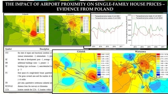
The studies analyzed the impact of two airports in Poland, i.e., Gdańsk and Warsaw, on the prices of single-family houses located in the airport’s vicinity. The airports are located in the central and northern part of Poland. Gdańsk Lech Walesa Airport is located 10 kilometers west of Gdańsk and Sopot and 23 km south of Gdynia, and occupies an area of 240 ha. Half of the Pomeranian Voivodeship population lives near the Gdańsk Airport (the Tri-City agglomeration). Gdańsk Lech Walesa Airport is the so-called alternate aerodrome to Warsaw airport. Warsaw Chopin Airport (IATA code: WAW; ICAO code: EPWA) is Poland’s largest airport, located about 8 km southwest from the centre of Warsaw. The airport occupies an area of over 680 ha. These airports’ interconnection and Warsaw’s and Gdańsk’s significance for Poland’s economic, political, and administrative systems have determined the choice of these airports for the research. Warsaw, with a population of almost 2 million, is Poland’s capital and an important city for business. Gdańsk together with Gdynia and Sopot form the so-called Tri-City with a population of almost 1 million. Gdańsk is an important seaport, too. Figure 1 and Figure 2 show the Gdańsk Lech Walesa Airport and Warsaw Chopin Airport locations, including the limited use area (LUA) visualization and the location of the single-family houses used to investigate sales transactions (for an explanation of the black spots, see Section 3.2).
Figure 1 and Figure 2 shows the impact ranges of the limited use areas’ (LUA) boundaries marked in pink. In Warsaw, the LUA is divided into zones Z1 and Z2, in Gdańsk, the LUA consists of the A and B Zones. The zones closer to the airport demonstrate higher airport noise levels in general. Areas located further (zone B or Z2) demonstrate no formal environmental noise standards exceedances for residential buildings and, therefore, there is also no obligation and necessity to improve the residential buildings’ acoustic parameters. These zones (B and Z2) are designated for other sensitive building types, e.g., nurseries, kindergartens, schools, hospitals, old people’s homes.
3.2. Data Description
In the research into the vicinities of Gdańsk Lech Walesa Airport and Warsaw Chopin Airport, the sale prices of single-family houses (typical, two-story, detached, semi-detached, and terraced buildings) were utilized. The research time horizon was 2013–2017. The sales price data were obtained from notarial deeds gathered in the Register of real estate prices and values of Gdańsk and Warsaw City Halls. The total data selected for analysis included 404 real estate transactions in the vicinity of Gdańsk Lech Walesa Airport and 292 transactions in the vicinity of Warsaw Chopin Airport. The spatial distribution of average unit prices (PLN/m2) of single-family houses located near Gdańsk and Warsaw airports are shown in Figure 3.
The single-family house price distribution (Figure 3) for properties located near the airports in Gdańsk and Warsaw is static in its nature. The price formation dynamic approach in years 2013–2017 is shown in Figure 4.
Both figures (Figure 3 and Figure 4), both in static and dynamic terms, demonstrate a much higher price level for single-family houses in Warsaw (up to a maximum of about 4250 USD/m2) than in Gdańsk (up to a maximum of about 2750 USD/m2). The prices of houses located in the limited use area (LUA) are generally lower than of those located outside LUA in both cities At the same time, there are a significant number of transactions with prices which diverge from the average (marked with green circles in Figure 4) for single-family houses located at a significant distance from airports (outside the LUAs). This may indicate the buyers’ real preferences for the housing market. Buyers accept high price levels, however, only for houses outside the LUAs of the examined airports.
Application of a classic multiple regression model, spatial autoregressive model, and geographically weighted regression models for our research requires additional descriptive variables in addition to the information on single-family houses sale prices and dates. Some data were acquired from the Real Estate Cadastre and the National Geodetic and Cartographic Resources in Gdańsk and Warsaw. Additional information on house attributes (e.g., usable building area, lot area, the technical condition of the building) was obtained by on-site observations and additional spatial information available online. Eventually, apart from the single-family houses price (PRICE) and the date of sale (DATE), the eight explanatory variables were adopted, including the distance from the runway in kilometers and a dummy variable denoting the in-LUA location. Concerning our previous research [32], the real estate sales transactions were verified for their suitability for analysis following the standards applicable to real estate valuation (mainly to investigate the market character of the transaction). The LS (location quality with four-grade assessment) variable was then removed from the database and the LUA (location outside or inside of limited use area) variable was quantified in binary form (dummy variable). The description of variables adopted for analysis is presented in Table 1.
Basic descriptive statistics of key variables used in data analysis are presented in Table 2.
3.3. Methods
Classic regression models are a commonly used tool for modelling the real estate market phenomena, in which parameter estimation is usually carried out with the use of ordinary least squares [60,61]. The general form of the linear multiple regression model can be presented as follows:
where y is the dependent variable, xi is the independent variable, while β0, βi are the model parameters.
The classic linear multiple regression model does not always produce satisfactory results due to the nature of the scales for the independent variable and the dependencies’ non-linearity [61]. Furthermore, multiple regression models do not take into account spatial correlations between variables, hence, both model parameters and the residual component are not a location function. Use of models in which spatial effects are directly taken into account may be the solution to this problem. They can be taken into account in various ways, i.e., by applying the spatial econometric model [62], spatially switching regression [63], random coefficient models [64], semi-logarithmic model using a row-standardized distance-based spatial weight matrix [65], or geographically weighted regression [66]. In addition to classical regression models, the spatial autoregression (SAR) and geographically weighted regression (GWR) models were used.
Many factors are shaping the real estate value and, as a result, its transaction prices; however, location plays a significant role. The location comprises all the related conditions, inter alia, the socio-economic and spatial factors related to the use of the space and accessibility, as well as factors related to local amenities as well as nuisances [67]. A similar real estate location should therefore correspond to similar transaction prices, which is the essence of spatial autocorrelation. The study of the spatial autocorrelation phenomenon usually requires the determination of spatial weights which represent spatial relations recorded in the form of a graph or a matrix. The selection of weight determination method largely depends on the nature of the analyzed phenomenon, as well as on additional information not included in the data pool [62]. If we assume that distance is the key element of real estate similarity, then Euclidean distances may be applied to the analysed real estate coordinates (centroids). Spatial autocorrelation measures can be of both global (determine the strength and nature of spatial autocorrelation for the entire set of units) and local character. The most commonly used measure of global spatial autocorrelation is Moran’s I statistics, of which the formula and testing principles can be found in many studies (including [68]). In the real estate market, it can be intuitively assumed that the spatial autocorrelation phenomenon should occur. However, transaction prices are influenced by factors not related to the location or related indirectly (e.g., development form and utilities). These factors’ impact on transaction prices can be determined by using statistical models, and the use of the spatial autocorrelation phenomenon can greatly improve quality.
Interdependencies or interactions on the real estate market may relate to the dependent variable, independent variables, as well as the random component [69]. The spatial autoregression is when these interactions relate to an endogenous variable. This means that this variable’s value in other locations affects this variable’s value in the analyzed location. If the interactions relate to a random component, there is the phenomenon of spatial autocorrelation of the model’s random component. Of course, these interactions may also apply to independent variables, i.e., situations where the independent variable’s shape in a given location is affected by the values of the exogenous variables from other locations, in which case this is a cross-sectional spatial regression. Depending on the type of spatial interaction, usually, two basic spatial regression models are used: the spatial lag model and the spatial error model [70,71].
- X—independent variable matrix,
- β—coefficients vector (model parameters),
- ε~N (0, σ2I)—an error vector of the model,
- Wy—defined as the spatially delayed dependent variable,
- ρ—the spatial autocorrelation coefficient.
If spatial autocorrelation does not occur (ρ = 0) then we obtain the classic linear multiple regression model. However, if the regression models’ residues are spatially correlated, some variables of a spatial character can be included in the model. The impact of other variables which cannot be included in the model will be expressed in the form of residues [73]. This means that the global autocorrelation relation is included in the form of model errors. The general form of the spatial error model is as follows [72]:
λ is the spatial autocorrelation coefficient, while Wε is a spatially delayed error. This should be interpreted as the mean error from neighboring locations, while ξ is an independent model error.
The use of SAR models is particularly justified when prices are shaped by continuous variables which characterize environment conditions (e.g., pollution, road or air-traffic noise, level of urban greenery saturation) [74,75]. Besner [76] demonstrated that the application of autoregressive models significantly improved prediction accuracy. The detailed solution to the problems associated with the SAR models’ construction and testing is presented by Anselin and Arbia [69,71,72,77].
There are many ways to solve the problem of including the spatial structure of the studied phenomenon in regression models, described in the literature in detail [69,78]. One of the ways is to assign a weight to observations which, due to their space location, may theoretically have a greater impact on the studied phenomenon than the other. This can be expressed with the use of geographically weighted regression (GWR). The GWR model can be formulated as follows [66]:
where (ui, vi) determines the location expressed in ui and vi coordinates. The GWR model parameters’ estimation is similar to classic models, however, location-dependent observation weights are taken into account:
where W(ui, vi) is a diagonal weights matrix: the weights are a function of the distance between the coordinate-specified location (ui, vi) and the location of each point the observations were made in. This matrix takes a diagonal form whose elements can be calculated based on a spatial kernel. To determine the weights, functions similar in shape to the Gaussian distribution are most often used, e.g., in the form of a bisquare kernel function [79]. As a result of the GWR model use, several areas determined by the estimated parameters are obtained. The value diversity of these parameters in space indicates the local variability impact of the dependent variables on the independent variable, and thus, the spatial heterogeneity of the studied phenomenon [66]. Because the parameters are not estimated at every space point, but only at selected points, a local variability at any point can be determined by spatial interpolation, and the result can be presented in the form of Isarithmic maps. The GWR model’s detailed estimation and verification principles are provided by, inter alia, Brunsdon et al. [80], Leung et al. [81] and Lu et al. [82]. They emphasize that usually the geographically weighted regression results better reflect the relations in the real estate market compared to global models. Furthermore, they indicate that the spatial diversity of the estimated regression parameters often indicates the non-stationary impact nature of non-spatial features on transaction prices. Examples of geographically weighted regression models use for transaction prices analyses in the real estate market are quoted by inter alia McCord et al. [83]. The example of Belfast indicates that space can be key in explaining price volatility. Similarly, Manganelli et al. [84], using the example of the housing market in the city of Potenza, built a GWR model to identify homogeneous areas and to define the marginal contribution that a single location (outlined by these areas) gives to the market value of the property. In other cases [85], the GWR model is used to study the spatial heterogeneity of the relations between property size and price. The studies carried out in major Chinese cities are particularly noteworthy [86]. The use of GWR models for the forward-looking changes analysis in real estate prices under the influence of not only physical factors directly related to real estate, but also the immigrant population, gross domestic product, and housing investment, was presented. It can be generalized that there has been a growing interest in the use of geographically weighted regression for housing market research in recent years [87,88].
The single-family house prices dynamics in 2013–2017 in Gdańsk and Warsaw were included in our research by analysing time series. The essence of the time series analysis is the search for real estate prices fluctuations over time, including the detection of certain properties’ regularities or substantial changes influenced by significant external factors. Time is not the cause of changes for a given phenomenon per se, however, it is controlled for to diagnose changes in this phenomenon. Important variables are selected from all elements set for a given phenomenon and a general time series form is developed, maintaining the time-related hierarchy. The series usually start from the oldest to the most recent events. According to Milo [89], a time series is a numerical sequence of observation results ordered in a time sequence. The time series illustrates the studied phenomenon’s evolution shaped by the influence of a large number of factors with different characteristics, strength and time of impact [90]. There are the two main purposes for the time series structure analysis. One of the purposes is to explain the nature of the phenomenon represented by the observation sequence. The other is to predict future values. Both these objectives require a more or less formal identification and description of the time series components, i.e., causes (fluctuations) quantifying which ones cause specific variability of the studied phenomenon [91]. The time-series study in real estate prices encounters a fundamental research problem related to the high non-uniformity level of real estate which are aggregated. The end result measures may show a large variation (high variability) in individual sub-periods since the average or median values in subsequent subperiods are determined based on completely independent (in relation to the previous period) price populations. Hence the need to refine the time series of property prices. This study uses Fast Fourier Transform (FFT) which utilizes four points of window (more in: [92,93]).
4. Results of Research and Discussion
4.1. Time Series Analysis
The research assumed the real estate price dynamics difference for properties located in limited use areas (in zones A and B in Gdańsk, and in Z1 and Z2 in Warsaw) and for real estate located outside these zones. Table 3 presents descriptive statistics for single-family house prices in and outside the limited use areas in Gdańsk and Warsaw.
The low number of analysed transactions (N = 81) in both Gdańsk and Warsaw for single-family houses located in the limited use area of the respective airports did not make it possible to determine the monthly average values for particular periods. Therefore, quarterly average levels for the examined periods were determined. The number of analysed transactions outside the LUAs in both cities is much higher, which indicates that the housing market is more active in these areas. Figure 5 shows the designated time series of quarterly average for real estate prices in 2011–2019.
Determination of the development tendency and price change direction is possible if time series are developed and then seasonal and random fluctuations are compensated by a time series refinement procedure. The time series refinement procedure allows for a significant reduction of the noise amplitude of the original raw data course and, as a result, the maintenance of real estate prices’ original trend, as well as reducing the data non-uniformity problem in particular periods. The refinement process was carried out with the use of Fast Fourier Transform FFT with the use of a 4-level window (Points of Window) and 0.00137 cut-off frequency. Figure 6 shows the refined time series in 2013–2017 in Gdańsk and Warsaw.
The 2013–2017 period in Gdańsk demonstrates a clear tendency for higher average quarterly prices for single-family houses located outside the LUA. Only in 2014, the average quarterly prices in the limited use areas approached the single-family houses price level outside the LUA. The quarterly percentage difference between average prices in the LUA and outside the LUA in Gdańsk ranges from −1.45% to 19.39%. Assuming that the average values’ level is about 9%, the prices of single-family houses outside the LUA of Gdańsk Lech Walesa Airport are higher by c.a. USD 68/m2 (273 PLN/m2). The 2013–2017 period in Warsaw demonstrates a clear tendency for higher average quarterly prices for single-family houses located outside the LUA. The quarterly percentage difference between average prices in the LUA and outside the LUA in Warsaw ranges from 33.23% to 46.44%. Assuming that the average values’ level is about 39%, the prices of single-family houses outside the LUA of the Warsaw Chopin Airport are higher by c.a. 424 USD/m2 (1698 PLN/m2).
4.2. Statistical and Geo-Spatial Analysis
The analysis of the airports’ impact on the real estate market utilized several statistical models, including both OLS regression models, as well as spatial autoregression models (SAR) and geographically weighted regression models (GWR). The paper hypothesizes that airports’ locations affect prices in airports’ surroundings. Classic regression models usually ignore the spatial aspect or take it into account indirectly, hence the use of spatial models designed to help identify sources of price formation, with particular emphasis on the airport-operation related factors.
The natural logarithm of a real estate price—a developed plot with a single-family house—was adopted as the dependent variable. The log-linear model form makes it possible to take into account the relative relation (percentage) and at the same time eliminates the adverse effect of large price differentiation. Estimation results of the OLS model for the area around the Lech Walesa Airport in Gdańsk and the area around the Chopin Airport in Warsaw are shown in Table 4.
For the OLS model developed for the area around Gdańsk airport, the statistically significant parameters with a significance level of less than 0.05 are found with the DATE, SZ, PU, PD, and LUA variables. Interestingly, the model shows that parameters related to the size of the property (PU, PD) are more important for the unit prices development rather than its technical and functional condition (STU). The parameter estimation results indicate that there is no reason to reject the hypothesis that there is no significant relationship between the distance from the runway (RUNWAY) and transaction prices. This may mean that the lower living comfort associated with airport proximity and airport noise is compensated by other factors that have a positive impact on prices (including infrastructure and a well-developed public transport network). The parameter attached to the LUA variable is noteworthy. This parameter is significant at the 0.027 significance level and its value is −0.131. This means that unit prices in the limited use area around Lech Walesa airport are slightly more than 12% lower than real estate prices outside the area. Therefore, the model suggests that prices may abruptly change at the area border, rather than in a linear manner associated with increasing distance.
For the OLS model developed for the transactional data around the Warsaw airport, the statistically significant parameters with a significance level of less than 0.05 are found with the SZ, DB, PU, and LUA variables. Although the RUNWAY variable proved to be the stimulus as expected, the parameter value of this variable was 0.068, at a significance level of 0.232, which means that there is no reason to reject the hypothesis that there is no impact of the distance from the runway on prices. The parameter value of the LUA variable of −0.345 is extremely important information. After conversion (e−0.345 − 1), this indicates that prices in the limited use area around the Fryderyk Chopin airport in Warsaw are approximately 29% lower than real estate prices outside this area.
Unfortunately, neither of the models shows a great fitting level measured by the coefficient of determination. Therefore, OLS modelling results should be approached with great caution. This problem may arise from the failure to take into account relevant spatial factors which affect prices. These factors are extremely difficult to identify. The problem’s solution may be the use of models which take into account spatial relationships directly. Therefore, the study examined the possibilities of using spatial autoregression (SAR) models. The basis for SAR model construction is the assumption that there is a significant spatial autocorrelation between the dependent variable values. This autocorrelation was examined by determining the global Moran’s I statistics and verifying the lack of a spatial correlation hypothesis. In the global autocorrelation study, a spatial weight matrix determined on the inverse of distance was used. Figure 7 presents the Moran plot showing the relations between price logarithms and their spatially delayed values (standardized values were used for the purpose).
The Moran’s chart indicates a slightly greater spatial autocorrelation of data for the area around the Warsaw airport; this has been confirmed by the results presented in Table 5.
A significant positive global spatial autocorrelation was observed for both the area around the Gdańsk airport and the area around the Warsaw airport. This can be interpreted as follows—location similarity also means unit price similarity. The spatial autocorrelation occurrence may be an important premise for the spatial autoregression (SAR) models’ purposefulness. Spatial relations in spatial autoregression models may take the spatial delay model form or a spatial error model form. The Lagrange Multiplier (LM) test was thus performed to determine the correct model form. The test results are presented in Table 6.
The analysis demonstrates that the spatial error model (RLMerr is significant, the level of significance for RLMlag is higher than 0.05) is the correct one for the area around the airport in Gdańsk. The spatial delay model (RLMerr is irrelevant, while RLMlag is important) is an appropriate form of the spatial autoregression model for the area around the airport in Warsaw. Table 7 presents the results of the SAR models’ parameters estimation.
The preliminary SAR model assessment makes it possible to detect that they are much better data-fitted compared to OLS models. The residual standard error(RSE) may also prove that in OLS models it was 0.280 for Gdańsk and 0.473 for Warsaw. In SAR models, the deviation was 0.212 and 0.311, respectively. Both models indicate high positive spatial autocorrelation. In the case of the spatial error model for Gdańsk, the spatial autocorrelation coefficient for residuals was 0.908, in the spatial delay model for Warsaw the spatial autocorrelation coefficient for price logarithms was 0.965.
In the SAR model for Gdańsk, there is a greater number of significant parameters compared to the OLS model (furthermore, STU and DB variables parameters proved to be significant). It is worth noting that distance from the runway does not significantly affect prices, similar to the OLS model. This model indicates that the property being located in the limited use area does not significantly affect prices, either. At the same time, it is worth noting that the significant spatial autocorrelation assumption in some specific locations may not be met, e.g., in the case of real estate located near the limited use area’s border (in that case, adjacent properties sold may be located inside the LUA and outside the LUA).
In the Warsaw SAR model, the parameter values changed at the RUNWAY and LUA variables. This indicates that in this case, a significant part of the price logarithms’ variability was explained by spatial autocorrelation. The distance from the runway is a stimulus, similar to the OLS model. The parameter value at the RUNWAY variable indicates that prices decrease by approximately 11% with each kilometer away from the runway. According to the SAR model, the location in the limited use area results in a lower price decrease than in the OLS model. In this case, the price difference was about 10% (this results from the (e−0.111 − 1) × 100% = −10.5% conversion), however, with a 0.009 significance level.
Considering the specificity of the around-airports area and the diversity of factors which affect prices, the assumption that the same level of spatial autocorrelation exists throughout the analysed area may seem oversimplistic. Figure 8 presents the spatial distribution of local Moran statistics for both Gdańsk and Warsaw. The distribution may indicate the analysed area’s heterogeneity.
As it turns out, the interpretation of both the global OLS model and SAR models may not be unambiguous, especially when we consider RUNWAY and LUA’s impact on prices. There are clear high-price clusters in the analysed area, as well as areas with negative spatial autocorrelation, i.e., high- and low-price real estates are adjacent. Therefore, another hypothesis was put forward during the study—the airport’s impact is not uniform throughout the entire analysed area, which means that the impact of both distance from the runway and location in the limited use area may differ depending on the specific location. The use of geographically weighted regression models (GWR) may offer the solution to the problem of individual variables’ impact depending on the location.
The same variables set from the areas around Gdańsk and Warsaw airports were used for GWR modelling. The overall modelling results for both areas are shown in Table 8.
In the spatial analysis of the airports’ impact on prices, the DATE, RUNWAY, and LUA variables may be of particular importance. The spatial distribution of the parameter at the date of the transaction variable may indicate locations where the price change rate differs from the price change rate in neighboring areas—taking into account the airport location, this may lead to conclusions about the airport’s impact on the price-change trend. For the sake of interpretation clarity, this trend is presented as a percentage change on an annual basis. Figure 9 shows the spatial distribution of the three variables for the area around the airport in Gdańsk along with the distribution of the significance level.
The highest price-change trend value was recorded in the northwest and southeast parts of the analyzed area. Significant values (with a significance level lower than 0.05) relate to the ends of the limited use area. However, it can be concluded that the overwhelming area of significant price increase is located outside the LUA. This may be treated as indication that this area may in a way negatively affect prices. The result of the spatial analysis of the RUNWAY variable’s impact on prices is interesting. This variable is a price stimulus in the majority of areas and its impact decreases with distance. This parameter changes quite rapidly in the direction consistent with the shape of the limited use area’s boundaries. The significance distribution map indicates that the distance from the runway and thus the price change occurs only in the immediate airport vicinity and in limited housing estates areas located in the LUA vicinity. The values presented on the spatial distribution map of the parameter at the LUA variable can be interpreted as showing that a potential change in the limited use area boundaries would result in a change in prices corresponding to the parameter value in a given location. These values are positive in the southern part, while in the northern part, towards the city center, the impact is negative. The area is directly adjacent to the airport itself where the influence of the parameter related to the LUA variable is statistically significant. This area could potentially experience the negative effects of restrictions related to the introduction of a limited use area and maximum permitted aircraft noise.
Figure 10 shows the spatial distribution of parameter values at the DATE, RUNWAY, and LUA variables for the area around the airport in Warsaw along with the distribution of the significance level.
The spatial distribution of the variable at the date of the transaction indicates that there are significant price drops near the airport. As the distance from the airport grows, the rate of price decline decreases. At the ends of the limited use area, this trend is positive. It can therefore be concluded that there is a fundamental relationship between distance from the airport and the rate of price changes. The significance level of spatial distribution indicates that a significant, negative trend is primarily attached to areas within a c.a. 3 km radius from the airport. At the same time, it is not correlated with the limited use area’s boundaries’ shape. It can be concluded, based on the parameter value distribution at the RUNWAY variable, that the strength of influence of the distance from the runway decreases with distance, which means, for example, that the assumption of a linear nature of relations in the OLS and SAR model is not fully met. However, when attention is paid to the spatial distribution of the significance level, the parameter controlling the influence of the distance from the runway turns out to be statistically significant only in certain small areas which can be compared to islands. This may be related to the surrounding built-up nature, the occurrence of open areas and thus, certain areas’ greater exposure to aircraft noise. The spatial distribution of the parameter at the LUA variable indicates primarily the possibility of price changes in areas at risk of aircraft noise. This parameter’s substantive interpretation is somewhat difficult to carry out because it indicates price differences within and outside the LUA, determined for data located in a radius equal to the bandwidth calculated based on the Akaike information criterion minimization (in this case the radius was 7930 m). However, for the area around the Gdańsk airport, this may mean a price change accompanied by a potential change in the LUA boundaries. Based on the spatial distribution of the level of significance, it can be concluded that the area of significant impact of this variable extends primarily west of the airport and covers strongly urbanized areas towards the city centre.
Analysis of the airport vicinity’s impact with the use of GWR models makes it possible both to identify factors which affect the price level and to determine their spatial distribution and to indicate locations where this impact is significant. The GWR models’ validity is also confirmed by a comparative analysis of the criteria fit of particular models used in the research. Table 9 presents selected criteria for OLS, SAR, and GWR model assessment.
The least-squares fit of GWR models is much better than of OLS models, especially for the area around the Warsaw airport. Additionally, information criteria (AIC) indicate that spatial models reflect the analyzed relations better than global OLS models. It is also worth noting that the GWR models have the smallest residual standard error (RSE). The analyses lead to the conclusion that geographically weighted regression models are purposefully used to analyze the airport vicinity’s impact on prices of residential real estate.
5. Remarks and Conclusions
Ensuring people’s welfare and satisfying people’s needs are the basic goals of socio-economic development. The sense of security realized by ownership of a house or apartment is a basic social need. Following the sustainable development principle, a balance between economic, environmental, and social objectives should be sought. The positive external effects of airport operations include infrastructural development and economic growth (jobs, tourism, and airport-related services). The negative external effects mainly include aircraft noise, real estate use restrictions, and air pollution. The sum of positive and negative externalities determines the net effect of being in the airport’s vicinity. In social terms, airport location is an important, decision-making factor for all those buying a house or an apartment. The real estate price has a measurable effect on such decisions. The price reveals all internal and external attributes which explain the price differentiation reasons in the housing market. Many previous studies (extensively discussed in the chapter with the literature review) on the airport impact and airport-related nuisances have focused on the determination of the relations between noise or air pollution and property prices. We believe that our important achievement is to show that lower prices on the real estate market are primarily a consequence of location within the LUA area, taking into account all the factors influencing their value, both positive and negative (not only aircraft noise).
This research, however, analyzed the airport impact on the prices of single-family houses located in airport-adjacent areas. This impact limit is determined by the limited use areas around the airports in Gdańsk and Warsaw. The conducted research is an extension and supplementation of the results of analyses conducted by Cellmer et al. [32]. First of all, the adoption of two airports for analysis allowed to compare and confront the results and to draw more universal conclusions. Moreover, the adoption of the same set of variables in each analyzed model allowed for a direct comparative assessment of the impact of location in the limited use areas (LUA) of both airports on real estate prices. This research utilized the time series analysis and a classic multiple regression model, spatial autoregressive model, and geographically weighted regression models. Despite the fundamental differences in research methodology of these models, similar results were obtained for Gdańsk and Warsaw. The time series analysis demonstrated that average prices for single-family houses within the limits set by the limited use areas (LUA) are lower than the average prices observed outside the LUAs. In Gdańsk, the difference is about 9%, while in Warsaw it is about 39%. Similar results were obtained with the use of statistical modelling. The use of the multiple regression model (OLS) showed that the prices of houses located in a limited use area around Gdańsk Lech Walesa Airport are c.a. 12% lower. In the case of Warsaw Chopin Airport, house prices are lower by approximately 29% compared to property prices outside this area. However, the OLS model has a low fit to empirical data (thus results are not fully reliable). Including spatial effects in the regression model leads to slightly different results. In the spatial autoregression model (SAR), the result of the studied relations for Gdańsk is not statistically significant (p-value = 0.460), while for Warsaw the location impact inside the LUA is about 10% with the significance level of 0.009. The results of the geographically weighted regression model (GWR) used in the study take into account the spatial heterogeneity of prices phenomenon. The authors are aware that the airport’s impact is not homogeneous throughout the area (the high- and low-price clusters are adjacent). Thus, the GWR model results do not take into account one price difference value (as in the OLS model and the SAR model), but value ranges. At the same time, the result of the (LUA [%]) model presented in Figure 9 and Figure 10 must be interpreted together with the statistical significance indications (p-value). The geographically weighted regression model for Gdańsk Lech Walesa Airport’s surrounding areas in places where it is statistically significant (north-central part of the LUA) produces dominant values ranging from −7% to −19%. For the area around Warsaw Chopin Airport, the GWR model in places where it is statistically significant (northeastern part of the LUA) produces values ranging from −16% to −36%. This indicates that there are areas around the airport where the negative effects of its proximity prevail, which is reflected in lower transaction prices. According to the observations, there may be two main reasons for the above-mentioned significant discrepancies between the airports in Gdańsk and Warsaw which were analysed. First, the negative impact of an airport’s neighborhood may be related to the airport size. Passenger traffic at the Chopin Airport in Warsaw is over three times greater than that at the airport Lech Walesa Airport in Gdańsk (in 2018, 17.8 million and 4.9 million passengers, respectively). The location and specificity of the environment may be another reason. The Gdańsk airport became operational in 1974 at a relatively large distance from the city’s developed areas. The area around the airport became a built-up area later on. The Warsaw airport was commissioned in 1934. The end of the 20th century and the beginning of the 21st century marked the intensive urbanization period in Warsaw, which ultimately led to the fact that the airport has been surrounded by urban tissue. At the same time, there is only a few kilometers’ distance from the Warsaw airport to the city centre. In the case of the Lech Walesa Airport in Gdańsk, the several-kilometre distance to the city center includes the urban forest zone.
The result summary leads to the conclusion that the use of time-series analyses and a classic multiple regression model, spatial autoregressive model, and geographically weighted regression models demonstrated airports’ negative impact on the prices of single-family houses located in limited use areas in Gdańsk and Warsaw. Caution should be exercised when interpreting the research results. Lower prices in the airport’s LUA mean that negative externalities outweigh the positive ones, so the total net effect of airport proximity is negative. Because the research purpose was to determine the combined effect of the positive and negative factors resulting from the airport proximity on real estate prices, this cannot be used to assess possible compensation for value reduction related to the restrictions introduced in LUAs. The studies do not prove in particular that the introduction of limited use areas affects the price level of single-family houses. In more general terms, the assumptions have been confirmed that broadly defined market boundaries outside the LUA, which are, however, still recognized as those in the vicinity of the airport, may be considered by buyers as being in the airport’s vicinity. This, therefore, may be considered an important factor which explains the single-family house price differences and also affects decisions regarding a house purchase or sale. The authors believe that the research concept adopted in this article should be further verified for other airport areas, as well as being extended to other types of real estate. There is an additional important further research area—a new methodological approach towards determination of the external border outside the LUA of the analysed market. The perspective of a neoclassical equilibrium model of the housing market functioning is generally accepted in empirical research. However, considering the significant location diversity of the real estate in question (inside and outside of LUAs), it might be necessary to segment the market for cause and effect inference to obtain two similar research sub-markets for analysis. In such case, it would be necessary to complement the house market perception which is now generally used in this type of research and perceived as homogeneous and limited to its features. Subjective features, i.e., market segmentation in relation to buyers’ housing preferences, should be included.
Author Contributions
Conceptualization, M.B., R.C. and M.G.; methodology, M.B. and R.C.; validation, M.B., R.C.; formal analysis, M.G.; investigation, M.B., R.C. and M.G.; resources, M.B., R.C.; data curation, M.B., R.C., M.G.; writing—original draft preparation, M.B., R.C. and M.G.; writing—review and editing, M.B., R.C. and M.G.; visualization, M.B., R.C.; supervision, M.B., R.C.; the participation of the first two authors is equal in value. All authors have read and agreed to the published version of the manuscript.
Funding
This research received no external funding.
Acknowledgments
The authors express sincere gratitude to the journal editor and the anonymous reviewers who spent their valued time to provide constructive comments and assistance to improve the quality of this paper.
Conflicts of Interest
The authors declare no conflict of interest.
References
- Hou, Y.; Long, R.; Zhang, L.; Wu, M. Dynamic Analysis of the sustainable development capability of coal cities. Resour. Policy 2020, 66, 101607. [Google Scholar] [CrossRef]
- Avesani, M. Sustainability, Sustainable development, and business sustainability. In Life Cycle Sustainability Assessment for Decision-Making; Ren, J., Toniolo, S., Eds.; Elsevier: Amsterdam, The Netherlands, 2020; pp. 21–38. [Google Scholar] [CrossRef]
- Laine, M. Meanings of the Term ‘sustainable development’ in finnish corporate disclosures. Account. Forum 2005, 29, 395–413. [Google Scholar] [CrossRef] [Green Version]
- Onishi, A. The world economy to 2015: Policy simulations on sustainable development. J. Policy Model. 2001, 23, 217–234. [Google Scholar] [CrossRef]
- Pawłowski, A. The sustainable development revolution. Probl. Sustain. Dev. 2009, 4, 65–76. [Google Scholar]
- Shulla, K.; Filho, W.L.; Sommer, J.H.; Salvia, A.L.; Borgemeister, C. Channels of collaboration for citizen science and the sustainable development goals. J. Clean. Prod. 2020, 264, 121735. [Google Scholar] [CrossRef]
- Visseren-Hamakers, I.J. The 18th sustainable development goal. Earth Syst. Gov. 2020, 100047. [Google Scholar] [CrossRef]
- Korhonen, J. Industrial ecology in the strategic sustainable development model: Strategic applications of industrial ecology. J. Clean. Prod. 2004, 12, 809–823. [Google Scholar] [CrossRef]
- Lundvall, B.-A.; Johnson, B. The learning economy. J. Ind. Stud. 1994, 1, 23–42. [Google Scholar] [CrossRef]
- Kirchgässner, G. Homo Oeconomicus: The Economic Model of Behaviour and Its Applications in Economics and Other Social Sciences; Springer Science & Business Media: Berlin, Germany, 2008; Volume 6. [Google Scholar]
- Vriend, N.J. Rational behavior and economic theory. J. Econ. Behav. Organ. 1996, 29, 263–285. [Google Scholar] [CrossRef]
- Bennett, P.; Howard, N. Rationality, emotion and preference change drama-theoretic models of choice. Eur. J. Oper. Res. 1996, 92, 603–614. [Google Scholar] [CrossRef]
- Becchetti, L.; Bruni, L.; Zamagni, S. Chapter 9—The theory of homo reciprocans. In The Microeconomics of Wellbeing and Sustainability; Becchetti, L., Bruni, L., Zamagni, S., Eds.; Academic Press: Cambridge, MA, USA, 2020; pp. 271–293. [Google Scholar] [CrossRef]
- White, M.D. Can homo economicus follow kant’s categorical imperative? J. Socio-Econ. 2004, 33, 89–106. [Google Scholar] [CrossRef]
- Bastien, C.; Cardoso, J.L. From homo economicus to homo corporativus: A neglected critique of neoclassical economics. J. Socio-Econ. 2007, 36, 118–127. [Google Scholar] [CrossRef]
- Brzezicka, J.; Wiśniewski, R. Homo oeconomicus and behavioral economics. Contemp. Econ. 2014, 8, 353–364. [Google Scholar] [CrossRef] [Green Version]
- Górka, K.; Thier, J. Wdrażanie koncepcji rozwoju zrównoważonego i trwałego. Aura 2019, 5, 8–12. [Google Scholar]
- Barrett, A.B. Stability of zero-growth economics analysed with a minskyan model. Ecol. Econ. 2018, 146, 228–239. [Google Scholar] [CrossRef]
- Cahen-Fourot, L.; Lavoie, M. Ecological monetary economics: A post-keynesian critique. Ecol. Econ. 2016, 126, 163–168. [Google Scholar] [CrossRef]
- Kaiser, F.G.; Henn, L.; Marschke, B. Financial rewards for long-term environmental protection. J. Environ. Psychol. 2020, 68, 101411. [Google Scholar] [CrossRef]
- Górka, K.; Poskrobko, B.; Radecki, W. Ochrona Środowiska; PWE: Warszawa, Poland, 2001; p. 205. [Google Scholar]
- Gobbo, J.A.; Busso, C.M.; Gobbo, S.C.O.; Carreão, H. Making the links among environmental protection, process safety, and industry 4.0. Process. Saf. Environ. Prot. 2018, 117, 372–382. [Google Scholar] [CrossRef] [Green Version]
- Xu, J.; Liu, T. Technological Paradigm-based approaches towards challenges and policy shifts for sustainable wind energy development. Energy Policy 2020, 142, 111538. [Google Scholar] [CrossRef]
- Mouri, T.; Iba, H. Hydrogen-Absorbing Alloys with a large capacity for a new energy carrier. Mater. Sci. Eng. A 2002, 329, 346–350. [Google Scholar] [CrossRef]
- Michałowski, A. Usługi środowiska w świetle bezpieczeństwa ekologicznego. Ekon. Śr. 2015, 4, 10–24. [Google Scholar]
- Trojanek, R.; Huderek-Glapska, S. Measuring the Noise Cost of Aviation—The association between the limited use area around warsaw chopin airport and property values. J. Air Transp. Manag. 2018, 67, 103–114. [Google Scholar] [CrossRef]
- Ventura, P.; Zazzi, M.; Rossetti, S.; Carra, M. Urban development and airports in northern and central Italy: Main trends and a focus on parma giuseppe verdi case study. Transp. Res. Procedia 2020, 45, 914–921. [Google Scholar] [CrossRef]
- Hakfoort, J.; Poot, T.; Rietveld, P. The regional economic impact of an airport: The case of amsterdam schiphol airport. Reg. Stud. 2001, 35, 595–604. [Google Scholar] [CrossRef]
- Percoco, M. Airport activity and local development: Evidence from Italy. Urban Stud. 2010, 47, 2427–2443. [Google Scholar] [CrossRef]
- Dzhambov, A.M.; Dimitrova, D.D. Urban Green spaces’ effectiveness as a psychological buffer for the negative health impact of noise pollution: A systematic review. Noise Health 2014, 16, 157. [Google Scholar] [CrossRef]
- Lawton, R.N.; Fujiwara, D. Living with aircraft noise: Airport proximity, aviation noise and subjective wellbeing in england. Transp. Res. Part Transp. Environ. 2016, 42, 104–118. [Google Scholar] [CrossRef]
- Cellmer, R.; Bełej, M.; Konowalczuk, J. Impact of a vicinity of airport on the prices of single-family houses with the use of geospatial analysis. ISPRS Int. J. Geo-Inf. 2019, 8, 471. [Google Scholar] [CrossRef] [Green Version]
- Batóg, J.; Foryś, I.; Gaca, R.; Głuszak, M.; Konowalczuk, J. Investigating the impact of airport noise and land use restrictions on house prices: Evidence from selected regional airports in Poland. Sustainability 2019, 11, 412. [Google Scholar] [CrossRef] [Green Version]
- Habdas, M.; Konowalczuk, J. Cele i warunki skutecznej interwencji państwa w obszarach ograniczonego użytkowania portów lotniczych. Świat Nieruchom. 2018, 3, 5–16. [Google Scholar] [CrossRef]
- Brueckner, J.K. Metropolitan airline traffic: Determinants and effects on local employment growth/BEBR No. 894. In BEBR Faculty Working Paper; University of Illinois at Urbana-Champaign: Champaign, IL, USA, 1982. [Google Scholar]
- Forsyth, P. Martin kunz memorial lecture. Tourism benefits and aviation policy. J. Air Transp. Manag. 2006, 12, 3–13. [Google Scholar] [CrossRef]
- Halpern, N.; Bråthen, S. Impact of airports on regional accessibility and social development. J. Transp. Geogr. 2011, 19, 1145–1154. [Google Scholar] [CrossRef]
- Wolfe, P.J.; Yim, S.H.L.; Lee, G.; Ashok, A.; Barrett, S.R.H.; Waitz, I.A. Near-airport distribution of the environmental costs of aviation. Transp. Policy 2014, 34, 102–108. [Google Scholar] [CrossRef] [Green Version]
- Barrett, S.R.; Britter, R.E.; Waitz, I.A. Global mortality attributable to aircraft cruise emissions. Environ. Sci. Technol. 2010, 44, 7736–7742. [Google Scholar] [CrossRef] [PubMed]
- Levy, J.I.; Woody, M.; Baek, B.H.; Shankar, U.; Arunachalam, S. Current and future particulate-matter-related mortality risks in the united states from aviation emissions during landing and takeoff. Risk Anal. 2012, 32, 237–249. [Google Scholar] [CrossRef]
- Mashhoodi, B.; Timmeren, A.V. Airport location in european airport regions: Five typologies based on the regional road network and land use data. Data Brief 2020, 29, 105317. [Google Scholar] [CrossRef] [PubMed]
- Diez, D.M.; Dominici, F.; Zarubiak, D.; Levy, J.I. Statistical Approaches for Identifying Air Pollutant Mixtures Associated with Aircraft Departures at Los Angeles International Airport. Available online: https://pubs.acs.org/doi/pdf/10.1021/es3007172 (accessed on 22 May 2020).
- Unal, A.; Hu, Y.; Chang, M.E.; Odman, M.T.; Russell, A.G. Airport related emissions and impacts on air quality: Application to the atlanta international airport. Atmos. Environ. 2005, 39, 5787–5798. [Google Scholar] [CrossRef]
- Sedoarisoa, N.; Desponds, D.; Dalmas, L.; Lavandier, C. Prix de l’immobilier et proximité de la plate-forme aéroportuaire de Paris–Charles-de-Gaulle (CDG). L’Espace Géographique 2017, 46, 61–78. [Google Scholar] [CrossRef] [Green Version]
- Espey, M.; Lopez, H. The impact of airport noise and proximity on residential property values. Growth Chang. 2000, 31, 408–419. [Google Scholar] [CrossRef]
- Trojanek, R.; Tanas, J.; Raslanas, S.; Banaitis, A. The impact of aircraft noise on housing prices in poznan. Sustainability 2017, 9, 2088. [Google Scholar] [CrossRef] [Green Version]
- Krajewska, M.; Pawłowski, K. Coherent land policy and land value. Geomat. Environ. Eng. 2019, 13. [Google Scholar] [CrossRef]
- Suksmith, P.L.; Nitivattananon, V. Aviation impacts on property values and management: The case of suvarnabhumi international airport. IATSS Res. 2015, 39, 58–71. [Google Scholar] [CrossRef] [Green Version]
- Cheung, T.K.-Y.; Wong, W.; Zhang, A.; Wu, Y. Spatial panel model for examining airport relationships within multi-airport regions. Transp. Res. Part Policy Pract. 2020, 133, 148–163. [Google Scholar] [CrossRef]
- Nguy, A.; Sun, C.; Zheng, S. Airport Noise and residential property values: Evidence from Beijing. In Proceedings of the 17th International Symposium on Advancement of Construction Management and Real Estate; Wang, J., Ding, Z., Zou, L., Zuo, J., Eds.; Springer: Berlin, Heidelberg, 2014; pp. 473–481. [Google Scholar] [CrossRef]
- Zambrano-Monserrate, M.A.; Ruano, M.A. Does environmental noise affect housing rental prices in developing countries? Evidence from Ecuador. Land Use Policy 2019, 87, 104059. [Google Scholar] [CrossRef]
- Winke, T. The Impact of aircraft noise on apartment prices: A differences-in-differences hedonic Approach for Frankfurt, Germany. J. Econ. Geogr. 2016, 17, 1283–1300. [Google Scholar] [CrossRef]
- Salvi, M. Spatial Estimation of the impact of airport noise on residential housing prices. Swiss J. Econ. Stat. 2008, 144, 577–606. [Google Scholar] [CrossRef] [Green Version]
- Li, M.M.; Brown, H.J. Micro-neighborhood externalities and hedonic housing prices. Land Econ. 1980, 56, 125–141. [Google Scholar] [CrossRef]
- Zheng, X.; Peng, W.; Hu, M. Airport noise and house prices: A quasi-experimental design study. Land Use Policy 2020, 90, 104287. [Google Scholar] [CrossRef]
- Tsui, W.H.K.; Fung, M.K.Y. Causality between business travel and trade volumes: Empirical evidence from Hong Kong. Tour. Manag. 2016, 52, 395–404. [Google Scholar] [CrossRef]
- Tomkins, J.; Topham, N.; Twomey, J.; Ward, R. Noise versus Access: The impact of an airport in an urban property market. Urban Stud. 1998, 35, 243–258. [Google Scholar] [CrossRef]
- Ozkurt, N.; Sari, D.; Akdag, A.; Kutukoglu, M.; Gurarslan, A. Modeling of noise pollution and estimated human exposure around istanbul atatürk airport in Turkey. Sci. Total Environ. 2014, 482, 486–492. [Google Scholar] [CrossRef] [PubMed]
- Rahayu, Y.E.; Ahyudanari, E.; Pratomoadmojo, N.A. Land use development and its impact on airport access road. Procedia-Soc. Behav. Sci. 2016, 227, 31–37. [Google Scholar] [CrossRef] [Green Version]
- Isakson, H. The Review of Real Estate Appraisals Using Multiple Regression Analysis; Social Science Research Network: Rochester, NY, USA, 1998. [Google Scholar]
- Benjamin, J.; Guttery, R.; Sirmans, C.F. Mass appraisal: An introduction to multiple regression analysis for real estate valuation. J. Real Estate Pract. Educ. 2004, 7, 65–77. [Google Scholar] [CrossRef]
- LeSage, J.P. An Introduction to spatial econometrics. Rev. Déconomie Ind. 2008, 123, 19–44. [Google Scholar] [CrossRef] [Green Version]
- Anselin, L. Spatial dependence and spatial structural instability in applied regression analysis. J. Reg. Sci. 1990, 30, 185–207. [Google Scholar] [CrossRef]
- Longford, N.T. Random Coefficient Models; Oxford Statistical Science Series; Oxford University Press: Oxford, NY, USA, 1994. [Google Scholar]
- Andersson, H.; Jonsson, L.; Ögren, M. Property prices and exposure to multiple noise sources: Hedonic regression with road and railway noise. Environ. Resour. Econ. 2010, 45, 73–89. [Google Scholar] [CrossRef] [Green Version]
- Fotheringham, A.S.; Brunsdon, C.; Charlton, M. Geographically Weighted Regression: The Analysis of Spatially Varying Relationships; John Wiley & Sons: Hoboken, NJ, USA, 2003. [Google Scholar]
- Basu, S.; Thibodeau, T.G. Analysis of spatial autocorrelation in house prices. J. Real Estate Financ. Econ. 1998, 17, 61–85. [Google Scholar] [CrossRef]
- Cliff, A.D. Spatial Autocorrelation; Pion: London, UK, 1973. [Google Scholar]
- Anselin, L. Spatial Econometrics: Methods and Models; Springer Science & Business Media: Berlin, Germany, 2013; Volume 4. [Google Scholar]
- Páez, A.; Scott, D.M. Spatial statistics for urban analysis: A review of techniques with examples. GeoJournal 2004, 61, 53–67. [Google Scholar] [CrossRef]
- Arbia, G. Spatial Econometrics: Statistical Foundations and Applications to Regional Convergence; Advances in Spatial Science Springer: Heidelberg, Germany, 2006. [Google Scholar] [CrossRef]
- Anselin, L. Spatial externalities, spatial multipliers, and spatial econometrics. Int. Reg. Sci. Rev. 2016. [Google Scholar] [CrossRef]
- Osland, L. An application of spatial econometrics in relation to hedonic house price modeling. J. Real Estate Res. 2010, 32, 289–320. [Google Scholar]
- Bourassa, S.; Cantoni, E.; Hoesli, M. Predicting house prices with spatial dependence: A comparison of alternative methods. J. Real Estate Res. 2010, 32, 139–159. [Google Scholar]
- Conway, D.; Li, C.Q.; Wolch, J.; Kahle, C.; Jerrett, M. A spatial autocorrelation approach for examining the effects of urban greenspace on residential property values. J. Real Estate Finance Econ. 2010, 41, 150–169. [Google Scholar] [CrossRef]
- Besner, C. A Spatial autoregressive specification with a comparable sales weighting scheme. J. Real Estate Res. 2002, 24, 193–212. [Google Scholar]
- Anselin, L. Lagrange multiplier test diagnostics for spatial dependence and spatial heterogeneity. Geogr. Anal. 1988, 20, 1–17. [Google Scholar] [CrossRef]
- Haining, R.P.; Kerry, R.; Oliver, M.A. Geography, spatial data analysis, and geostatistics: An overview. Geogr. Anal. 2010, 42, 7–31. [Google Scholar] [CrossRef]
- Charlton, M.; Fotheringham, S.; Brunsdon, C. Geographically weighted regression. J. R. Stat. Soc. Ser. D 1998, 47, 431–443. [Google Scholar]
- Brunsdon, C.; Fotheringham, S.; Charlton, M. Geographically Weighted Regression as a Statistical Model; Working Paper; University of Newcastle-upon-Tyne: Newcastle, UK, 2000. [Google Scholar]
- Leung, Y.; Mei, C.-L.; Zhang, W.-X. Statistical tests for spatial nonstationarity based on the geographically weighted regression model. Environ. Plan. A 2000, 32, 9–32. [Google Scholar] [CrossRef]
- Lu, B.; Harris, P.; Charlton, M.; Brunsdon, C. The GWmodel R package: Further topics for exploring spatial heterogeneity using geographically weighted models. Geo-Spat. Inf. Sci. 2014, 17, 85–101. [Google Scholar] [CrossRef]
- McCord, M.; Davis, P.T.; Haran, M.; McGreal, S.; McIlhatton, D. Spatial variation as a determinant of house price: Incorporating a geographically weighted regression approach within the belfast housing market. J. Financ. Manag. Prop. Constr. 2012, 17, 49–72. [Google Scholar] [CrossRef]
- Manganelli, B.; Pontrandolfi, P.; Azzato, A.; Murgante, B. Using geographically weighted regression for housing market segmentation. Int. J. Bus. Intell. Data Min. 2014, 9, 161–177. [Google Scholar] [CrossRef]
- Lu, B.; Charlton, M.; Fotheringhama, A.S. Geographically weighted regression using a non-euclidean distance metric with a study on london house price data. Procedia Environ. Sci. 2011, 7, 92–97. [Google Scholar] [CrossRef] [Green Version]
- Yang, S.; Hu, S.; Li, W.; Zhang, C.; Torres, J.A. Spatiotemporal effects of main impact factors on residential land price in major cities of China. Sustainability 2017, 9, 2050. [Google Scholar] [CrossRef] [Green Version]
- Wu, H.; Jiao, H.; Yu, Y.; Li, Z.; Peng, Z.; Liu, L.; Zeng, Z. Influence factors and regression model of urban housing prices based on internet open access data. Sustainability 2018, 10, 1676. [Google Scholar] [CrossRef] [Green Version]
- Cellmer, R.; Belej, M.; Zrobek, S.; Kovač, M.Š. Urban land value maps—A methodological approach. Geod. Vestn. 2014, 58, 535–551. [Google Scholar] [CrossRef]
- Milo, W. Szeregi Czasowe; Państwowe Wydawnictwo Ekonomiczne: Warszawa, Poland, 1990. [Google Scholar]
- McDowall, D.; McCleary, R.; Bartos, B.J. Interrupted Time Series Analysis; Oxford University Press: Oxford, UK, 2019. [Google Scholar]
- Cox, D.R.; Gudmundsson, G.; Lindgren, G.; Bondesson, L.; Harsaae, E.; Laake, P.; Juselius, K.; Lauritzen, S.L. Statistical analysis of time series: Some recent developments (with discussion and reply). Scand. J. Stat. 1981, 8, 93–115. [Google Scholar]
- Rao, K.R.; Kim, D.N.; Hwang, J.J. Fast Fourier Transform-Algorithms and Applications; Springer Science & Business Media: Berlin, Germany, 2011. [Google Scholar]
- Liu, S.; Wang, Q. Studying contact stress fields caused by surface tractions with a discrete convolution and fast Fourier transform algorithm. J. Tri. 2002, 124, 36–45. [Google Scholar] [CrossRef] [Green Version]
Figure 1.
Localization of Gdańsk Lech Walesa Airport and limited use area (LUA).

Figure 2.
Localization of Warsaw Chopin Airport and limited use area (LUA).

Figure 3.
Spatial distribution of mean single-family house prices (PLN/sqm) around Warsaw Chopin Airport and Gdańsk Lech Walesa Airport.
Figure 3.
Spatial distribution of mean single-family house prices (PLN/sqm) around Warsaw Chopin Airport and Gdańsk Lech Walesa Airport.

Figure 4.
Dynamics of single-family house prices (PLN/m2) around Warsaw Chopin Airport (a) and Gdańsk Lech Walesa Airport (b) from 2013 to 2017.
Figure 4.
Dynamics of single-family house prices (PLN/m2) around Warsaw Chopin Airport (a) and Gdańsk Lech Walesa Airport (b) from 2013 to 2017.

Figure 5.
Time series of mean single-family house prices inside and outside the LUAs around Gdańsk Lech Walesa Airport (GDN) (a) and Warsaw Chopin Airport (WAW) (b) from 2013 to 2017 (quarterly).
Figure 5.
Time series of mean single-family house prices inside and outside the LUAs around Gdańsk Lech Walesa Airport (GDN) (a) and Warsaw Chopin Airport (WAW) (b) from 2013 to 2017 (quarterly).

Figure 6.
Smoothed time series of mean single-family house prices inside and outside the LUAs around Gdańsk Lech Walesa Airport (GDN) (a) and Warsaw Chopin Airport (WAW) (b) from 2013 to 2017 (quarterly).
Figure 6.
Smoothed time series of mean single-family house prices inside and outside the LUAs around Gdańsk Lech Walesa Airport (GDN) (a) and Warsaw Chopin Airport (WAW) (b) from 2013 to 2017 (quarterly).

Figure 7.
Moran’s scatterplot for the standardized Lnprice variable.

Figure 8.
Spatial distribution of local Moran statistics for the dependent variable Lnprice.

Figure 9.
Spatial distribution of selected parameters from the GWR model (Gdańsk).

Figure 10.
Spatial distribution of selected parameters from the GWR model (Warsaw).


Table 1.
Description of variables.
| Symbol | Description |
|---|---|
| STU | The state of repair and functional condition of a single-family house: to be demolished [1], (minus) intermediate [2], intermediate [3], (plus) intermediate [4], favorable [5]. |
| SZ | The state of development: poor [1], average [2], favorable [3]. |
| DB | Additional buildings: none [1], present [2]. |
| FZ | Building type: rowhouse [1], semi-detached house, end-of-terrace house [2], detached building [3]. |
| PU | Floor space of a single-family house: quantitative continuous area calculated as the product of the gross covered area and the number of stories, but taking into account the irregularity of solids. |
| PD | Plot area; quantitative continuous cadastral area. |
| RUNWAY | Distance from the runways in kilometers. |
| LUA | Location outside the LUA [0], location within the LUA [1]. |
Table 2.
Basic descriptive statistics for data.
| Gdańsk Lech Walesa Airport | Warsaw Chopin Airport | |||||||
|---|---|---|---|---|---|---|---|---|
| Variable | Min | Median | Max | Std. Dev | Min | Median | Max | Std. Dev |
| STU | 1 | 4 | 5 | 1.01 | 1 | 3 | 4 | 0.73 |
| SZ | 1 | 2 | 3 | 0.73 | 1 | 2 | 3 | 0.55 |
| DB | 1 | 1 | 2 | 0.28 | 1 | 1 | 3 | 0.57 |
| FZ | 1 | 1 | 3 | 1.35 | 1 | 2 | 3 | 0.77 |
| PU | 50 | 156.5 | 390 | 60.99 | 77 | 187.5 | 408 | 71.67 |
| PD | 73 | 535.5 | 2482 | 438.88 | 123 | 331.5 | 2000 | 306.12 |
| RUNWAY | 1.44 | 5.93 | 11.07 | 2.33 | 1.440 | 6.456 | 14.140 | 2.76 |
| LUA | 0 | 0 | 1 | 0.37 | 0 | 0 | 1 | 0.44 |
Table 3.
Descriptive statistics on prices of single-family houses inside and outside the LUAs around Gdańsk and Warsaw airports.
Table 3.
Descriptive statistics on prices of single-family houses inside and outside the LUAs around Gdańsk and Warsaw airports.
| Gdańsk Lech Walesa Airport | Warsaw Chopin Airport | |||
|---|---|---|---|---|
| Inside of LUA | Outside of LUA | Inside of LUA | Outside of LUA | |
| N total | 81.00 | 323.00 | 81 | 211 |
| Mean | 3198.27 | 3423.58 | 4352.968 | 6438.539 |
| Standard Deviation | 1070.56 | 1651.67 | 1786.527 | 3589.27 |
| SE of mean | 118.95 | 91.90 | 198.503 | 247.0955 |
| Variance | 1,146,091.81 | 2,728,005.81 | 3,191,680 | 1.29 × 10⁷ |
| Skewness | 0.56 | 1.47 | 1.24238 | 1.11348 |
| Kurtosis | 0.68 | 3.18 | 1.32478 | 0.86368 |
| Geometric Mean | 3017.61 | 3071.18 | 4043.029 | 5564.323 |
| Minimum | 1134.15 | 576.35 | 1704.55 | 1923.08 |
| Maximum | 6837.61 | 10,492.75 | 9717.95 | 19,107.39 |
Table 4.
Results of the ordinary least squares (OLS) model parameter estimation.
| Gdańsk Lech Walesa Airport | Warsaw Chopin Airport | |||||
|---|---|---|---|---|---|---|
| Estimate | Std. Error | p−Value | Estimate | Std. Error | p-Value | |
| Intercept | 8.575 | 0.242 | <0.001 | 8.693 | 0.290 | <0.001 |
| DATE | 0.009 | 0.003 | 0.008 | −0.004 | 0.002 | 0.123 |
| STU | −0.034 | 0.025 | 0.166 | −0.057 | 0.047 | 0.219 |
| SZ | 0.164 | 0.035 | <0.001 | 0.229 | 0.061 | <0.001 |
| DB | −0.120 | 0.079 | 0.131 | −0.205 | 0.053 | <0.001 |
| FZ | −0.032 | 0.019 | 0.095 | −0.080 | 0.053 | 0.131 |
| PU | −0.003 | 3.9 × 10⁻⁴ | <0.001 | 8.9 × 10⁻⁴ | 4.0 × 10⁻⁴ | 0.026 |
| PD | 2.0 × 10⁻⁴ | 6.0 × 10⁻⁵ | 0.001 | 2.1 × 10⁻⁴ | 1.3 × 10⁻⁴ | 0.095 |
| RUNWAY | −0.002 | 0.046 | 0.960 | 0.068 | 0.056 | 0.232 |
| LUA | −0.131 | 0.059 | 0.027 | −0.345 | 0.064 | <0.001 |
| RSE: 0.280, R2 = 0.374, Adj. R2 = 0.339. | RSE: 0.473, R2 = 0.213, Adj. R2 = 0.187. | |||||
Table 5.
Moran I statistic.
| Gdańsk Lech Walesa Airport | Warsaw Chopin Airport | |
|---|---|---|
| Global Moran’s I | 0.1932 | 0.4542 |
| Expectation | −0.0059 | −0.0035 |
| Variance | 0.0008 | 0.0005 |
| Global Moran I std | 6.7902 | 20.5190 |
| p-value | <0.001 | <0.001 |
Table 6.
Lagrange Multiplier diagnostics for spatial dependence.
| Gdańsk Lech Walesa Airport | Warsaw Chopin Airport | |||
|---|---|---|---|---|
| Stat | p-Value | Stat | p-Value | |
| LMerr | 69.930 | <0.001 | 261.260 | <0.001 |
| LMlag | 67.699 | <0.001 | 322.710 | <0.001 |
| RLMerr | 4.616 | 0.032 | 0.700 | 0.403 |
| RLMlag | 2.385 | 0.122 | 62.151 | <0.001 |
| SARMA | 72.316 | <0.001 | 323.410 | <0.001 |
Table 7.
General estimation results from spatial autoregression (SAR) models.
| Gdańsk Lech Walesa Airport (Error SAR) | Warsaw Chopin Airport (Lag SAR) | |||||
|---|---|---|---|---|---|---|
| Estimate | Std. Error | p-Value | Estimate | Std. Error | p-Value | |
| Intercept | 8.271 | 0.279 | <0.001 | 0.024 | 0.233 | 0.918 |
| DATE | 0.007 | 0.002 | 0.005 | −0.003 | 0.002 | 0.072 |
| STU | 0.065 | 0.024 | 0.006 | 0.045 | 0.031 | 0.142 |
| SZ | 0.089 | 0.027 | 0.001 | 0.113 | 0.040 | 0.005 |
| DB | −0.139 | 0.062 | 0.026 | −0.104 | 0.035 | 0.003 |
| FZ | −0.016 | 0.015 | 0.309 | −0.009 | 0.035 | 0.798 |
| PU | −0.004 | 3.1 × 10⁻⁴ | <0.001 | −0.002 | 2.6 × 10⁻⁴ | <0.001 |
| PD | 3.2 × 10⁻⁴ | 4.9 × 10⁻⁵ | <0.001 | 2.9 × 10⁻⁴ | 8.6 × 10⁻⁵ | <0.001 |
| RUNWAY | 0.008 | 0.044 | 0.845 | 0.107 | 0.037 | 0.004 |
| LUA | −0.042 | 0.057 | 0.460 | −0.111 | 0.042 | 0.009 |
| λ: 0.908, RSE: 0.212 | ρ: 0.965, RSE: 0.311 | |||||
Table 8.
General estimation results from geographically weighted regression (GWR) models.
| Gdańsk Lech Walesa Airport | Warsaw Chopin Airport | |||||||
|---|---|---|---|---|---|---|---|---|
| Variable | Min | Mean | Max | Std. Dev | Min | Mean | Max | Std. Dev |
| Intercept | 7.698 | 8.419 | 8.897 | 0.199 | 6.593 | 8.760 | 10.507 | 0.560 |
| DATE | −0.0002 | 0.009 | 0.015 | 0.003 | −0.018 | −0.003 | 0.010 | 0.006 |
| STU | −0.069 | 0.056 | 0.137 | 0.035 | −0.186 | 0.108 | 0.318 | 0.111 |
| SZ | 0.004 | 0.093 | 0.209 | 0.042 | −0.246 | 0.048 | 0.455 | 0.146 |
| DB | −0.335 | −0.154 | 0.243 | 0.145 | −0.309 | −0.043 | 0.248 | 0.092 |
| FZ | −0.072 | −0.027 | 0.005 | 0.013 | −0.541 | −0.042 | 0.097 | 0.117 |
| PU | −0.005 | −0.004 | 0.003 | 0.0004 | −0.006 | −0.003 | 0.0004 | 0.001 |
| PD | 0.0002 | 0.0004 | 0.0008 | 0.0002 | −0.0002 | 0.0006 | 0.002 | 0.0005 |
| RUNWAY | −0.053 | −0.009 | 0.095 | 0.032 | −0.228 | −0.009 | 0.257 | 0.059 |
| LUA | −0.437 | −0.003 | 0.444 | 0.168 | −0.795 | −0.181 | 0.395 | 0.059 |
| Local R2 | 0.325 | 0.660 | 0.723 | 0.051 | 0.406 | 0.585 | 0.841 | 0.115 |
| RSE: 0.194, R2: 0.682, Adj. R2: 0.339 | RSE: 0.256, R2: 0.761, Adj. R2: 0.681 | |||||||
Table 9.
Overview of diagnostic statistics for OLS, SAR and GWR models.
| Gdańsk Lech Walesa Airport | Warsaw Chopin Airport | |||||
|---|---|---|---|---|---|---|
| Parameter | OLS | SAR | GWR | OLS | SAR | GWR |
| R2 | 0.374 | - | 0.681 | 0.213 | - | 0.761 |
| Adj. R2 | 0.339 | - | 0.563 | 0.187 | - | 0.681 |
| AIC | 61.074 | −3.826 | 1.695 | 397.465 | 203.410 | 154.196 |
| BIC | 95.568 | 33.804 | 122.73 | 437.758 | 247.361 | 376,955 |
| LogLik | −19.537 | 13.912 | −75.502 | −187.733 | −89.702 | 32.568 |
| RSE | 0.280 | 0.212 | 0.194 | 0.473 | 0.311 | 0.256 |
© 2020 by the authors. Licensee MDPI, Basel, Switzerland. This article is an open access article distributed under the terms and conditions of the Creative Commons Attribution (CC BY) license (http://creativecommons.org/licenses/by/4.0/).
Share and Cite
MDPI and ACS Style
Bełej, M.; Cellmer, R.; Głuszak, M. The Impact of Airport Proximity on Single-Family House Prices—Evidence from Poland. Sustainability 2020, 12, 7928. https://doi.org/10.3390/su12197928
AMA Style
Bełej M, Cellmer R, Głuszak M. The Impact of Airport Proximity on Single-Family House Prices—Evidence from Poland. Sustainability. 2020; 12(19):7928. https://doi.org/10.3390/su12197928
Chicago/Turabian StyleBełej, Mirosław, Radosław Cellmer, and Michał Głuszak. 2020. "The Impact of Airport Proximity on Single-Family House Prices—Evidence from Poland" Sustainability 12, no. 19: 7928. https://doi.org/10.3390/su12197928
Note that from the first issue of 2016, this journal uses article numbers instead of page numbers. See further details here.