
A Regional View of Passenger Air Link Evolution in Brazil
by
 , , and
Vicente Aprigliano Fernandes
1,* ,
,
Ricardo Rodrigues Pacheco
2,
Elton Fernandes
2,
Manoela Cabo
3 and
Rodrigo V. Ventura
2,3 1
Escuela de Ingeniería de Construcción y Transporte, Pontifícia Universidad Católica de Valparaíso, Valparaíso 2362804, Chile
2
Production Engineering Program (COPPE), Federal University of Rio de Janeiro (UFRJ), Rio de Janeiro 21941-450, Brazil
3
Brazilian Institute of Geography and Statistics (IBGE), Rio de Janeiro 20031-170, Brazil
*
Author to whom correspondence should be addressed.
Sustainability 2022, 14(12), 7284; https://doi.org/10.3390/su14127284
Submission received: 6 May 2022
/
Revised: 10 June 2022
/
Accepted: 12 June 2022
/
Published: 14 June 2022
(This article belongs to the Section Sustainability in Geographic Science)
Abstract
:Passenger flows among cities, at both the domestic and international levels and in different countries and regions, have been studied for forecasting purposes. This paper seeks not a forecasting mechanism, but to understand, by analyzing passenger origins and destinations by Brazilian sub-region, how Brazil’s domestic air passenger network links have evolved. Using income, population, and fare price as inputs, and seats sold as output, air link performance is examined by data envelopment analysis to discuss the regional link of domestic passenger traffic in Brazil and its dynamics, considering two specific years. The findings indicate that, although the highest passenger flow density is concentrated in Brazil’s Southeast region, performance by emerging origins and destinations (O-Ds), such as those connecting the Northeast, display more substantial strength indices and advances (Malmquist analysis). The analysis of specific links was also important, which showed that important Brazilian airports are not necessarily more competent in generating trips. The Catch-Up indicator for innovation reveals the weak point in Brazil’s air transport network. Although some airports enjoy strong networkability, they do not correspond in passenger origin or destination strength.
1. Introduction
Passenger origin–destination (O-D) flow and its pattern are key components in transport companies’ business planning, mainly for airlines and airports. Its analysis is strategic for the best air route design, which can be organized through direct or connected flights. The actual O-D statistics of air passenger transport are not widely held available in the public domain, and as competition hardens, air fares fluctuate considerably. Such constraints make it difficult to formulate highly accurate models. Statistics identifying the reason for travel are also generally not publicly available. Passengers travel from one city to another on business, on holiday, to visit friends or relatives, and so on. Even without knowing the travel purpose, the passenger movement between different destinations can be investigated using a gravity model that examines the aggregate flow between any two cities connected by some common interest. It is interesting how network studies have been evolving, for example, by using mobile phone data [1] and through complex network analysis [2]. These kinds of studies are essential to understanding the role of cities’ hierarchy and transport hubs on the development of the territory from different scales of analysis: local, regional, national, and international.
In conceptual terms, gravity modeling uses the flow variable as a function of explanatory variables representing the mass and friction between any two points, and is also widely used to estimate price–income elasticities of demand for forecasting purposes [3]. Considering that the economy is a key driver of air travel demand [4], and that there is a strong correlation between economic development and air passenger demand [5,6], particularly in Brazil [7,8], this paper explores regional passenger flows by considering the O-Ds’ population and income, as well as the effectively commercialized fares for a significant sample of air travels in 2011 and 2016. In this matter, this research seeks to respond to the following question: How can we optimize the passengers flow on a given air route, given the income of the cities involved (O-Ds), their populations, and fares? By focusing on how air transport routes are able to induce passenger demand flows under an intra- and inter-regional view, and by highlighting bottlenecks regarding this issue, this research contributes to discussions on sustainable and territorially well-balanced economic development driven by the civil aviation industry, which are elements of development that are straightly related [9]. The analyzed period is justified by the fact that 2011 is the year in which the main airports in Brazil were conceded to private administration, whereas 2016 marks the consolidation of this concession process. This paper discusses the strength among air links, using data envelopment analysis (DEA) and Malmquist indices to show the dynamics of structural change. This kind of analysis is highly important to new Brazilian air transport market entrants endeavoring to establish themselves in Latin America’s largest market.
In addition, recently, there has been a radical shift away from a prosperity scenario, where air transport was growing, to a scenario where the economy is seeking avenues to recover from negative growth rates and disruptive phenomena, such as pandemics. Whereas the Brazilian annual geometric gross domestic product growth rate from 2011 to 2014 was 1.80%, from 2014 to 2016, it was −3.42% [10]. In an analogy between world crisis analysis [11] and the Brazilian case, the economic and political crisis observed in Brazil may be categorized as of major proportions, and domestic air passenger transport levels may take up to 36 months to recover. This could take even longer considering the outbreak of the Covid pandemic.
This paper is organized into seven sections. The first is concerned with contextualization and the study object. The second offers a review of selected literature, comprising the publications considered most relevant to the study. The third presents the methodology underpinning the discussion of findings. The fourth describes the data used in the methodology. The fifth briefly describes the Brazilian case. The sixth presents the findings from the analysis and discussion. The seventh and final section states the main conclusions from the analysis, and offers suggestions for future research.
2. Literature Review
Discussions on the origin–destination of air passenger traffic have been attracting researchers’ interest for some time now, including Derudder and Witlox [12], Grubesic et al. [13], and O’Connor and Fuellhart [14]. Derudder and Witlox [12], through a review of the literature, argue that future research should develop alternative ways of recording airline data with the aim of building more meaningful analyses, such as identifying the true origins and destinations of passengers, rather than just a specific segment of a trip.
Grubesic et al. [13] examined the emerging global hierarchy of the air transportation network by using the information of around 900 airline carriers from 2006, which considered 4650 origins and destinations. This study identified an increase in the complexity of the air networks in North America, Europe, and Asia. With a global perspective, O’Connor and Fuellhart [14] evaluate the relationship between cities´ hierarchy according to the Global and World City Project of Loughborough and air service characteristics. Results of this research show apparent differences between aircraft, airline size, and mode of operation depending on the city´s hierarchy within the global context.
Bhadra and Kee [15] analyzed the structure and dynamics of the main air transport markets in the United States, using quarterly series for the period between 1995–2006. The analysis focused on the origin–destination of commercial flights on the market segmented by the number of passengers transported per day (pax/day). They discovered that on thick markets (pax/day > 100), demand was relatively elastic to mean fares, whereas other markets displayed inelastic demand. Their results also showed that passenger trip O-Ds are generally income-inelastic. Pitfield et al. [16] made an empirical analysis of the fit between aircraft size and flight frequency on long-haul routes, considering traffic, airline behavior, and degree of competition. This study used 1990 data for nine routes on the North Atlantic market, where a considerable number of airlines operate in a competitive environment. Pitfield et al. used origin and destination data between European and United States airports, consisting of the number of passengers, flight frequency, and aircraft size. They concluded that, with increased passenger numbers, flight frequency was more likely to increase than aircraft size.
Puller and Taylor [17] examined individual flight ticket transactions for each itinerary on trunk routes of the United States domestic market in 2004. They used detailed data on ticket purchase dates and tariffs, origin and destination, flight number, and service class. Puller and Taylor concluded that airlines charged lower fares for similar flights depending on the day of the week, and that this phenomenon suggested a day-of-purchase price discrimination mechanism. Fageda and Flores-Fillol [18] examined air service provision on thin routes, comparing the United States market with those of the European Union, using origin–destination data between airports and others. Their analyses focused on the impact of two major innovations in the air transport industry: regional jet technology and low-cost airlines. Fageda and Flores-Fillol concluded that regional services provided higher flight frequency at higher fare prices, whereas low-cost services offered cheaper fares at the cost of lower flight frequencies.
Mumbower et al. [19] estimated flight price elasticity using an on-line database and the corresponding aircraft seat maps. These elasticities were estimated considering the number of reservations on the flight and how many days prior to departure the booking was made. Their findings indicated that price elasticity varied with the day of the week when the reservation was made, the time of day of departure, and competitors’ promotional sale dates. They showed that airlines could use these detailed price elasticity estimates, among other things, to forecast promotions. Luttmann [20] analyzed the reasons that may lead an airline to charge different one-way and return fares on the same route, depending on the point of origin of the trip, which is a case of directional price discrimination. For that purpose, he used data on airline passenger roundtrip ticket prices and origins and destinations obtained from the US Department of Transportation, as well as regional economic data, the reason for travel, and so on. He found significant evidence of income-related directional price discrimination, that is, airlines charged higher fares to passengers originating in cities with higher mean incomes.
Mohammadian et al. [21] examined the Australian domestic aviation market, using monthly data from 2004 to 2015 for 21 routes connecting eight cities. The aim was to investigate the relationship between demand per flight and capacity variables, such as frequency, aircraft size, load factor, etc. The results suggested that competition led to more flights, smaller aircraft, lower load factors, and more available seats in the markets studied. They also concluded that city socioeconomic parameters, such as population and employment rate, influenced flight demand more strongly on long-haul routes. Oliveira et al. [22] evaluated the effects of a series of determinants on air traffic network concentration and its possible decoupling relative to social and economic activity concentrations. They used air passenger, gross domestic product, and population for defining a concentration decoupling index. Their analysis discussed the relation of the decoupling and concentration indices with air passengers, international tourism, oil cost, slot constraints, airline competition, and socioeconomic events. Urban and Hornung [23], mapping causalities of airline dynamics, identified key elements for long-haul flight competition, which are the generation of transatlantic air transport demand, passenger choice, and airline ticket price and fleet development. Oliveira and Oliveira [24] showed that a Brazilian airline focusing on the regional flights segment conquered many monopoly positions across the country, strengthening its profitability.
The literature concerning airline passenger flows has focused on estimating forecasting models for better operational planning and scheduling by airlines. The studies generally consider the passengers’ behavior related to economic and situational variables, considering only the travel segments (instead of the actual origin and destination). This kind of simplification in the analysis opens a research gap, namely the potential profit earned by airlines as the result of changing market conditions. Furthermore, it is important to develop research related to intra- and inter-regional air traffic in order to understand, in terms of performance, the internal dynamics of air traffic in countries with continental dimensions, such as Brazil.
3. Materials and Methods
3.1. Methodology
In emerging economies with continental-sized domestic markets, such as Brazil, China, Russia, and others, the internal passenger traffic between their sub-regions assumes more complex characteristics, requiring a better understanding both of these flows and of the different regional particularities. This study applied a methodology for analyzing regional flows in terms of performance and structural change over a given period. This approach considers a different perspective regarding the elements that make up the independent variables of a forecast function, examining their explanatory power to determine the volume of passengers on a given route. The regional analysis will make it possible to identify the level of performance, in terms of passenger flows, for each region of the country, as well as the interregional interactions.
The methodology comprised three stages. The first involved organizing, describing, and cleaning the available data to suit the study purpose. At this stage, the sample for analysis was defined. The second stage involved calculating and analyzing the efficiency indices of the air links using DEA. In the third, Malmquist indices were calculated, and their variations were examined to reveal a structural change in the links. The analyses covered both the total movement and the intra- and interregional O-Ds.
DEA analysis considered each O-D individually, but overall efficiency indices for the sample of O-Ds were used here, by Brazilian sub-region. That is, these indices were calculated for each region. The overall performance index was expressed by weighted means for individual O-Ds. This result gave cluster means in relation to the efficiency frontier in each year. The result was a number from 0 to 1, where 1 meant that the O-D or cluster was at the efficiency frontier.
Dynamic performance analysis used the means from the Malmquist analysis. These represented the movement of efficiencies for specific characteristics and changes specific to an O-D or cluster. Malmquist analysis yields indices of change that vary around 1, where values of less than 1 mean the characteristic is deteriorating, a value of 1 means stagnation, and values greater than 1 represent progress. The cluster means from both the DEA and the Malmquist indices were calculated using means weighted by the number of passengers for each O-D in that cluster. This weighting is important, because the O-Ds had differing market shares. As the analysis covered a five-year period, it was important to take growth in demand as a reference point, because small efficiency gains might be insufficient to explain air transport growth. The distinction between intra- and inter-regional passenger flows is strategic for the development of the airline sector, and for the formulation of policies for strengthening and regulating the sector.
Considering the O-Ds’ managerial dimensions as inputs, and passengers processed as output, DEA depicted the best performance at each O-D and the overall situation of domestic air transport as a whole. The output maximization approach proved more appropriate to the study problem, because one of airlines’ main objectives is to maximize the passenger flow. Moreover, dynamic analysis was conducted using balanced panel data for the two years, 2011 and 2016.
DEA is a non-parametric method designed to measure the performance of a firm, organization, program, etc., i.e., whatever is produced by a decision-making unit (DMU). Charnes et al. [25] presented the various formulations developed for the DEA approach. In this study, the main issue was the organizations’ output potential. Given that the study object comprised O-Ds of differing sizes, the model chosen was the output-oriented approach using a variable return to scale (VRS). The proposed model, known as output-oriented BCC, involved the primal of the linear programming problem in Equation (1).
where: X is the vector of inputs used by the DMUs; Y is the vector of quantities produced (outputs) by the DMUs; ε is the infinitesimal non-Archimedean constant that assures that no input or output is assigned zero weight; s+ and s− are the slack vectors, respectively, of the outputs and inputs; ϕ is a scalar variable that represents the possible radial increase to be applied to all outputs so as to obtain the values of the projected outputs; and λ is the vector whose optimal values form a combination of units that make up the performance of the DMU under study, thus setting a direction by which to identify the sources of inefficiency in this DMU.
An O-D’s efficiency rating at any given moment is a static value. Malmquist analysis was used to reflect the O-D’s dynamic behavior in relation to the efficiency frontier from 2011 to 2016. The Malmquist index was used because it allows efficiency change to be decomposed into dimensions that are useful for understanding O-D performance. Authors have used different nomenclatures for these dimensions. The original study by Malmquist [26] decomposed efficiency change into components, as described by Coelli et al. [27], Färe et al. [28], Ray and Desli [29], and others. This study used the Malmquist total factor efficiency index (MI) decomposition proposed by Ray and Desli [29] for the VRS output-oriented DEA model. Ray and Desli decomposed the MI into three components. Equation (2) shows the MI for two years, 2011 and 2016. Its components are catch-up (CU) and frontier shift (FS) for the VRS, and the scale component (SEC).
where:
where:
(x0, y0)t represents the position of the O-D considered in period t, by way of its inputs and outputs;
δt represents the O-D’s efficiency index in period t for the variable return to scale frontier in period t; and
σt represents the O-D’s scale efficiency in relation to the frontier in period t.
The DEA and Malmquist parameters were weighted by the number of seats sold on the O-D. This weighting was important to prevent trends in the simple means of the country sub-region efficiency indicators, which might return disproportional measurements when small links had greater indicators than high passenger-density links, and vice versa. The analyses were conducted using mean values at the intra- and interregional levels. Although DEA was conceived to analyze production performance, this paper uses a formulation of a demand function, seeking to show how best O-D socioeconomic conditions and link price result in air transport link demand.
3.2. Case Study
Brazil occupies a geographical area of 8.5 million km2, making it the country with the fifth-largest territory in the world, after Russia, Canada, China, and the United States. In 2018, it also had the fifth largest population (209 million), according to World Bank figures. Its economy ranked seventh, with a GDP of around 3.388 trillion Int $ (PPP $—international dollar) in 2017 [30]. However, in 2015, Brazil ranked only 74th in per capita GDP (about 8670 Intl $), a long way from the group of countries classified as developed—as was also the case with other countries with large territories and significant GDPs, such as China, India, and Russia. Brazil is a federative republic comprising 26 states and the Federal District (the country’s capital), and is organized into five administrative regions: North (N), Southeast (SE), Midwest (MW), Northeast (NE), and South (S). Each Brazilian state has one municipality where the state capital is located. Brazil has 5570 municipalities, of which 309 had populations of more than 100,000 in 2016 [10]. This is a size that can be considered attractive for airline operations, especially when the city is more than 100 km from cities that already have airports. Despite this potential, only 90 cities were found to have airports operating regular flights in both 2011 and 2016. That fact seems to be connected with Brazil’s low per capita income combined with the concentration of the total GDP in the Southeast region.
Table 1 shows the distribution of GDP, population (POP), and GDP per capita according to the Brazil’s five regions. All monetary values, in Reais (Brazilian currency), presented in this study are in constant 2016 values, corrected by the National Extended Consumer Price Index (IPCA), the country’s official inflation rate. Note that, although the SE region’s share in GDP declined by 2.24 percentage points (p.p.), the SE continued to predominate quite clearly as the country’s economic center, accounting for more than 50% of all income and about 42% of the total population. The MW region, meanwhile, comprising a smaller percentage of the population, returned a higher per capita income than the SE. Two factors account for this situation: the first is that Brazil’s export-oriented agricultural and livestock production is concentrated in the MW, and the second is that the nation’s capital is located in this region. The NE region performed best in an increased share of GDP (a variation of more than 0.93 p.p.). Fernandes et al. [31] showed that this was the region that prospered most in service GDP, meaning that this region’s airports performed best in networkability. However, the NE is the region with the lowest per capita GDP in Brazil. Although the N and MW regions account for large portions of Brazil’s total area, they hold a smaller part of the population.
In the nomenclature used in this study, “passengers” (PAX) is synonymous with seats sold. Note, in Table 1, that the SE region’s share in all variables declined, although it continued to predominate by a considerable margin as the country’s economic powerhouse. The NE region performed best as regards growth in share of PAX.
Among the main economic activities in the NE region, tourism is particularly notable for its recent performance, and for its relevance in terms of income and employment generation. Silva et al. [32] present a hierarchy of 50 Brazilian airports associated with tourism, 38% of which are in the NE region, 20% in the MW, 18% in the N, 12% in the S, and 12% in the SE. Accordingly, the rising gross value of the service sector in the NE region is closely related to the tourism industry, whereas in the MW, the service sector’s gain in gross value correlates with growth in the region’s agribusiness sector. These data show that tourism plays a significant, but not predominant, role in PAX movement in the MW. The sample used in this study encompasses the main municipalities served by airports. The results for this group of cities better reflect the behavior of air transport in Brazil than the general statistics, since it represents the main economic centers of the country—a source of demand flows for air travel, and historically more sensitive to changes in the economic or political scenario.
3.3. Data
Air transport O-D databases are scarce in the field of air transport research [33,34,35,36]. It is thus common practice to use samples in related analyses. The data used in this study originated in microdata from the National Civil Aviation Agency (ANAC) (https://www.anac.gov.br/assuntos/dados-e-estatisticas/microdados-de-tarifas-aereas-comercializadas, accessed on 5 May 2022), which show the volume of tickets purchased on each trip, i.e., from origin to destination, by the price paid and by month. For the purpose of analysis, these data were transformed into annual values of O-D movement and weighted means of prices paid by O-D. According to the ANAC, these data represent about 50% of the total movement, because the database does not include tickets purchased under mileage programs or specific agreements between purchasers and airlines. The data on domestic airfares apply to all tickets sold. The GDP and POP figures for the main municipalities served by the trip origin and destination airports were obtained from Brazilian Institute of Geography and Statistics (IBGE).
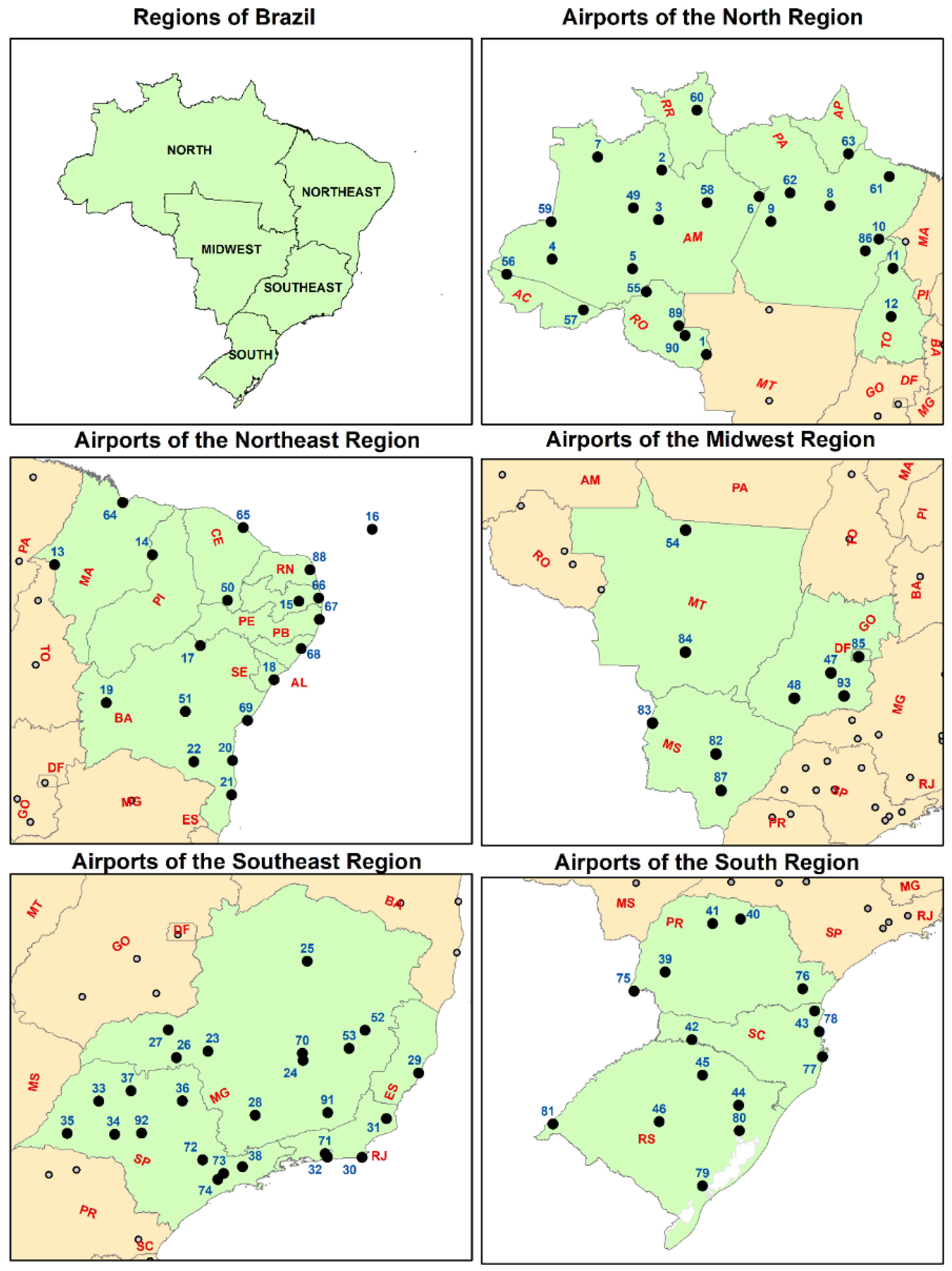
The database is directional, i.e., it considers outward and returns tickets separately. Each direction has a specific price. The links considered are those existing in 2011 and 2016, so that Malmquist analysis indices can be calculated. Links with an annual demand of at least 52 tickets were considered, so as not to include occasional ticket purchases as links. The data relate to the 26 state capitals, the national capital, 63 regional cities, and three of the state capitals (Belo Horizonte, Rio de Janeiro, and São Paulo, Brazil) with two airports each, totaling 93 airports that were operating in both 2011 and 2016. Within the specifications of the sample, 3133 O-Ds present in both years were validated. Appendix A contains a map of Brazil’s regions (Figure A1), showing the location of the airports covered by the study, and, in Table A1, the ICAO codes for the airports, the cities relating to each airport, and the name and abbreviation of each state.
The analytical model had five inputs and one output. The output is the number of seats purchased from one origin to a given destination. The inputs are the GDP and POP of the municipality of origin and destination municipality, and average ticket price weighted by tickets sold (TICK) in the years in question. Table 2 shows the correlation between output and inputs of the DEA model considered for analysis. As ticket prices vary inversely with passenger demand, this variable was transformed to its reciprocal, as suggested by Bowlin [37], in order to implement the DEA in such a manner as to guarantee the isotonicity of the variables.
Table 3 shows the descriptive statistics for the variables considered for analysis in this study. From Table 3, it can be seen that the standard deviations of the variables are quite large, revealing a significant variety of situations, ranging from low-density and/or short-haul links to high-density and long-haul links. Distances between airports in Brazil can be greater than 4000 km, as between Cruzeiro do Sul, in AC state, and João Pessoa, in PB state. There are 16 towns in the sample with fewer than 100,000 inhabitants; these are small, isolated localities, of tourist or strategic interest to the country. One example is Fernando de Noronha, an island and protected environment in the east of the NE region, whose economic activity is fundamentally tourism. Another example is Coari, in AM state in the N region, an isolated locality in the Amazon Forest, where there is significant production of natural gas. Data for GDP (in million Reais) and POP (in thousands of the population) relate to the 90 cities in the sample. The statistics used for the remaining variables refer to the 3133 O-Ds.
4. Results
Table 4 shows the results of the DEA and Malmquist analysis of the intra-regional links. It can be seen that only a small number of O-Ds were at the efficiency frontier—39 and 23, respectively, in 2011 and 2016—of a total of 690. In all, 20 O-Ds were at the efficiency frontier in both years. The regions returned CUs of 0.70 to 0.74, indicating a uniform decline in performance as regards this indicator of innovation. The SE and NE regions displayed FS improvements, the SE’s being the most significant (FS = 1.25). SEC remained relatively stagnant in all regions, ranging from 0.97 to 1.01. Overall, intra-regional air transport performance declined, with MI from 0.62 (MW) to 0.88 (SE). Table 4 also shows that from 690 O-Ds, 245 had MIs improved (35.51%); this happens mainly in the SE and NE regions, where FS were 1.25 and 1.07, respectively.
Overall, the analysis showed that in the intra-regional dimension, the indicator for innovation (CU) was most strongly connected with a diminished performance by O-Ds. From 690, 673 O-Ds had CU < 1 (97.54%). Meanwhile, the indicator for scale (SEC) stagnated, reflecting no variations in the regional structures. Although FS did advance in the SE and NE regions, those advances were insufficient to overcome the decline indicated by CU in these regions, leading to MI < 1. In the S and N regions, FS was nearly stagnant, and MI was thus influenced basically by the deterioration in CU. The MW region showed deteriorating FS, which led, in turn, to greater degradation indicated by CU, leaving the region with lower MI. The SE region’s performance, because of a good FS result (1.25), was the least affected in total efficiency, represented by MI.
Table 5 shows the results of the DEA and Malmquist analysis of the interregional O-Ds, where regular domestic air passenger transport flows are largest in Brazil, about 66% of the passenger sample. Although the O-Ds were further from the efficiency frontier than in the intra-regional cases, the indicators of improvement from the Malmquist analysis were much more promising. The considerable number of O-Ds involving the SE region (55% of the total) attests to this region being the main origin or destination of inter-regional passengers. The SE region O-Ds accounted for more than 50% of intra-regional passenger movement (Table 4). As in the intra-regional dimension, only a small number of O-Ds defined the efficiency frontier. Of the 52 O-Ds that were at the frontier in at least one of the study years, 32 were there in 2011, and 35 in 2016. Of these, 15 were at the frontier in both years. All regions had some O-D at the efficiency frontier. The inter-regional O-Ds that moved away from the efficiency frontier least were SE–NE and S–SE, which also comprised the links with the greatest number of passengers. However, total efficiency declined in both, with MI indicators equal to 0.88. The O-Ds with greatest performance improvements (MI > 1) were SE–N, S–NE, and S–N, among which the S region was conspicuous for improvement in total efficiency (MI = 1.15, 1.26, and 1.42). Poor O-D performance, as in the case of intra-regional O-Ds, can be associated primarily with the indicator for innovation, CU, which varied from 0.66 to 0.77. The indicator that displayed most overall improvement was FS. The indicator for scale (SEC) remained largely close to stagnant. Most (56%) of the inter-regional O-Ds returned an MI greater than 1, indicating an endeavor to improve the total efficiency in most of the O-Ds.
From Table 5, it can also be seen that the main improvements observed in the FS indicator did not occur on the highest-density passenger links, which were, in decreasing order of number of passengers, SE–NE, S–SE, and SE–MW.
5. Discussion
The intra-regional and inter-regional results obtained seem consistent with the particularities, recent trends, and economic dynamics of each of the Brazilian regions. Taking the discussion presented by Ter Wal and Boschma [38] about the influence of networks on the development of regional economies, together with the intra-regional results given here, we may infer that the SE region offers suitable social and economic conditions for increasing O-D efficiencies, particularly in connections with state capital cities, such as São Paulo, Rio de Janeiro, Belo Horizonte, and Vitoria. These cities have significant GDP, and greater population density and diversity of economic activities, enabling the “social network” to be more resilient [31]. As such, the connections with them, given the variety of economic opportunities available in the region, are better able to withstand regional economic crises. However, the industry does not seem to have made proper use of inter-regional potential. The S region shares a characteristic with the SE region, in that it accounts for the second-largest share of Brazil’s GDP [10]. As such, it offers suitable regional economic conditions for improving the MI for certain air links. The opposite effect can be seen in relation to the N region, which has the smallest share of national GDP, which is reflected in lesser diversity and intensity of economic activities and dynamics within the region, as well as in no improvement in the MI for intra-regional air links, whereas better prospects do exist at the inter-regional level, primarily in links with the S and SE regions.
The intra-regional result for the MW region seems to be related to the importance of agri-business to the region [39]. As was observed by Giuliani and Bell [40], with regard to the knowledge and technology network connected with wine production in Chile, which has little connectivity on a local or regional scale, i.e., it is an isolated network concentrated within the wine-producing companies or those that connect with agents outside the “natural” proximity zone (in other regions of Chile), this same process may be occurring with air traffic in the MW region, reflecting the stagnation or degradation of connections in the MW. At the inter-regional level, the O-Ds relating to this region returned the lowest MI values of the set (0.76, 0.85, and 0.86).
After the SE, it is the NE region that has benefited most from domestic tourism [41]. It should also be stressed that Bahia (BA) is the state with the largest GDP in the region [10], especially in the tertiary sector, primarily tourism. Unlike what happens in the MW region, the tourism-related service sector cuts across various other sectors and embodies more significant relations of geographical proximity. This strengthens the production chain of local and regional tourism, which influence factors from everyday leisure activities through to tourism activities in other places within the area of influence of the region’s tourism network, particularly the state of BA (where Salvador and Porto Seguro are located), as can be observed in the NE region’s intra-regional results. However, although one of the best-performing ODs in terms of total efficiency relates to the NE (S–NE), the set of higher inter-regional traffic density O-Ds (SE–NE) does not perform satisfactorily and deserves attention from air transport operators.
6. Conclusions
The present research investigates the degree of robustness of the domestic passenger air transport network in Brazil, using a regional analysis of the flow of travelers’ origin and destination. The sample selected for analysis comprises the period when the important economic changes experienced by the civil aviation industry in the country became more evident. Furthermore, although not random, the sample analyzed allows us to infer a general profile of the most relevant passenger flows for airline planning purposes.
The intra- and inter-regional analyses show that even though similarities exist, the various O-Ds differ in terms of performance, resilience, and potential. The weighted grouping of intra- and inter-regional indicators for the O-Ds give a more synthetic view of the travel generation efficiency in Brazil. Although the SE region returned better performance indicators at both intra- and inter-regional levels, other regions performed better in a number of other dimensions. Better performance indicators can be connected with major economic differences and population concentration, rather than with improvement in O-Ds. With only three inter-regional exceptions (S–N, S–NE, and SE–N), the MI indicators showed that airlines in Brazil have not managed to take advantage of the demand potential of domestic passenger O-Ds. The domestic airlines’ weak point was revealed by the CU indicator, one reason for which may be the lack of secondary airports in Brazilian state capitals, which hinders supply flexibility. Another may be the entry barriers facing new competitors, which are still rather high. Catching up and forging ahead calls for a more innovative attitude on the part of domestic airlines in Brazil.
Brazil’s most recent family budget survey, covering the years 2017 and 2018 [10], showed that the share of spending on domestic air transport had almost doubled in Brazilian family budgets, as compared with the previous survey for 2008 and 2009 (from 0.32% to 0.57%). However small this percentage may be, this statistic suggests that Brazilian households, in general, recognize the utility of air transport in their lives. Moreover, this utility tends to be even greater in remote or isolated areas, such as those located in the Brazilian Amazon, situated in the N region. However, the results point out that airlines are still not showing themselves capable of taking advantage of this market opportunity by offering products and services to expand the number of air travels in the country, so that they return satisfactory efficiency indicators. In other words, the contribution of the aviation industry in Brazil to the integration of markets, people, and economic development is still below its potential level. Deepening this analysis and providing new elements for this discussion will be the object of future research, which can be developed based on the findings presented here.
Author Contributions
Conceptualization, V.A.F.; methodology, V.A.F., R.R.P. and E.F.; validation, V.A.F., R.R.P. and E.F.; formal analysis, V.A.F., R.R.P. and E.F.; investigation, V.A.F., R.R.P. and E.F.; data curation, R.R.P., E.F., M.C. and R.V.V.; writing—original draft preparation, V.A.F., R.R.P. and E.F.; writing—review and editing, V.A.F., R.R.P., E.F., R.V.V. and M.C.; visualization, V.A.F., R.R.P. and E.F.; supervision, V.A.F.; project administration, V.A.F.; funding acquisition, V.A.F. All authors have read and agreed to the published version of the manuscript.
Funding
The APC was funded by Escuela de Ingeniería de Construcción y Transporte, Pontificia Universidad Católica de Valparaíso.
Acknowledgments
The authors would like to thank the editor and anonymous reviewers for their insightful comments and suggestions.
Conflicts of Interest
The authors declare no conflict of interest.
Appendix A
Figure A1.
Location of airports in Brazil, by state and region.


Table A1.
Airports in each city, state, and region (IDs relate to Figure A1).
Table A1.
Airports in each city, state, and region (IDs relate to Figure A1).
| ID | ICAO | CITY | STATE | REGION |
|---|---|---|---|---|
| 85 | SBBR | Brasília | Distrito Federal (DF) | MIDWEST (MW) |
| 47 | SBGO | Goiânia | Goiás (GO) | |
| 48 | SWLC | Rio Verde | ||
| 93 | SBCN | Caldas Novas | ||
| 82 | SBCG | Campo Grande | Mato Grosso do Sul (MS) | |
| 83 | SBCR | Corumbá | ||
| 87 | SBDO | Dourados | ||
| 54 | SBAT | Alta Floresta | Mato Grosso (MT) | |
| 84 | SBCY | Várzea Grande | ||
| 68 | SBMO | Maceió | Alagoas (AL) | NORTHEAST (NE) |
| 19 | SNBR | Barreiras | Bahia (BA) | |
| 20 | SBIL | Ilhéus | ||
| 21 | SBPS | Porto Seguro | ||
| 22 | SBQV | Vitória da Conquista | ||
| 51 | SBLE | Lencóis | ||
| 69 | SBSV | Salvador | ||
| 50 | SBJU | Juazeiro do Norte | Ceará (CE) | |
| 65 | SBFZ | Fortaleza | ||
| 13 | SBIZ | Imperatriz | Maranhão (MA) | |
| 64 | SBSL | São Luís | ||
| 15 | SBKG | Campina Grande | Paraíba (PB) | |
| 66 | SBJP | Santa Rita | ||
| 16 | SBFN | Fernando de Noronha | Pernambuco (PE) | |
| 17 | SBPL | Petrolina | ||
| 67 | SBRF | Recife | ||
| 14 | SBTE | Teresina | Piauí (PI) | |
| 88 | SBSG | Natal | Rio Grande do Norte (RN) | |
| 18 | SBAR | Aracaju | Sergipe (SE) | |
| 56 | SBCZ | Cruzeiro do Sul | Acre (AC) | NORTH (N) |
| 57 | SBRB | Rio Branco | ||
| 2 | SWBC | Barcelos | Amazonas (AM) | |
| 3 | SWKO | Coari | ||
| 4 | SWEI | Eirunepé | ||
| 5 | SWLB | Lábrea | ||
| 6 | SWPI | Parintins | ||
| 7 | SBUA | São Gabriel da Cachoeira | ||
| 49 | SBTF | Tefé | ||
| 58 | SBEG | Manaus | ||
| 59 | SBTT | Tabatinga | ||
| 63 | SBMQ | Macapá | Amapá (AP) | |
| 8 | SBHT | Altamira | Pará (PA) | |
| 9 | SBIH | Itaituba | ||
| 10 | SBMA | Marabá | ||
| 61 | SBBE | Belém | ||
| 62 | SBSN | Santarém | ||
| 86 | SBCJ | Parauapebas | ||
| 1 | SBVH | Vilhena | Rondônia (RO) | |
| 55 | SBPV | Porto Velho | ||
| 89 | SBJI | Ji-Paraná | ||
| 90 | SSKW | Cacoal | ||
| 60 | SBBV | Boa Vista | Roraima (RR) | |
| 11 | SWGN | Araguaína | Tocantins (TO) | |
| 12 | SBPJ | Palmas | ||
| 29 | SBVT | Vitória | Espírito Santo (ES) | SOUTHEAST (SE) |
| 23 | SBAX | Araxá | Minas Gerais (MG) | |
| 24 | SBBH | Belo Horizonte | ||
| 25 | SBMK | Montes Claros | ||
| 26 | SBUR | Uberaba | ||
| 27 | SBUL | Uberlândia | ||
| 28 | SBVG | Varginha | ||
| 52 | SBGV | Governador Valadares | ||
| 53 | SBIP | Santana do Paraíso | ||
| 70 | SBCF | Confins | ||
| 91 | SBZM | Juiz de Fora | ||
| 30 | SBCB | Cabo Frio | Rio de Janeiro (RJ) | |
| 31 | SBCP | Campos dos Goitacazes | ||
| 32 | SBRJ | Rio de Janeiro | ||
| 71 | SBGL | Rio de Janeiro | ||
| 33 | SBAU | Araçatuba | São Paulo (SP) | |
| 34 | SBML | Marília | ||
| 35 | SBDN | Presidente Prudente | ||
| 36 | SBRP | Ribeirão Preto | ||
| 37 | SBSR | São José do Rio Preto | ||
| 38 | SBSJ | São José dos Campos | ||
| 72 | SBKP | Campinas | ||
| 73 | SBGR | Guarulhos | ||
| 74 | SBSP | São Paulo | ||
| 92 | SBAE | Bauru | ||
| 39 | SBCA | Cascavel | Paraná (PR) | SOUTH (S) |
| 40 | SBLO | Londrina | ||
| 41 | SBMG | Maringá | ||
| 75 | SBFI | Foz do Iguaçu | ||
| 76 | SBCT | São José dos Pinhais | ||
| 44 | SBCX | Caxias do Sul | Rio Grande do Sul (RS) | |
| 45 | SBPF | Passo Fundo | ||
| 46 | SBSM | Santa Maria | ||
| 79 | SBPK | Pelotas | ||
| 80 | SBPA | Porto Alegre | ||
| 81 | SBUG | Uruguaiana | ||
| 42 | SBCH | Chapecó | Santa Catarina (SC) | |
| 43 | SBJV | Joinville | ||
| 77 | SBFL | Florianópolis | ||
| 78 | SBNF | Navegantes |
References
- Zhang, W.; Fang, C.; Zhou, L.; Zhu, J. Measuring megaregional structure in the Pearl River Delta by mobile phone signaling data: A complex network approach. Cities 2020, 104, 102809. [Google Scholar] [CrossRef]
- Zhang, W.; Zhu, J.; Zhao, P. Comparing World City Networks by Language: A Complex-Network Approach. ISPRS Int. J. Geo-Inf. 2021, 10, 219. [Google Scholar] [CrossRef]
- Brons, M.; Pels, E.; Nijkamp, P.; Rietveld, P. Price elasticities of demand for passenger air travel: A meta-analysis. J. Air Transp. Manag. 2002, 8, 165–175. [Google Scholar] [CrossRef] [Green Version]
- Zhang, F.; Graham, D.J. Air transport and economic growth: A review of the impact mechanism and causal relationships. Transp. Rev. 2020, 40, 506–528. [Google Scholar] [CrossRef]
- Tong, T.; Yu, E. Transportation and economic growth in China: A heterogeneous panel cointegration and causality analysis. J. Transp. Geogr. 2018, 73, 120–130. [Google Scholar] [CrossRef]
- Tolcha, T.D.; Bråthen, S.; Holmgren, J. Air transport demand and economic development in sub-Saharan Africa: Direction of causality. J. Transp. Geogr. 2020, 86, 102771. [Google Scholar] [CrossRef]
- Cabo, M.; Fernandes, E.; Pacheco, R.R.; Pires, H. Economic Growth Relations to Domestic and International Air Passenger Transport in Brazil. Int. J. Transp. Veh. Eng. 2018, 12, 1475–1480. [Google Scholar]
- Aprigliano Fernandes, V.; Pacheco, R.R.; Fernandes, E.; Cabo, M.; Ventura, R.V.; Caixeta, R. Air Transportation, Economy and Causality: Remote Towns in Brazil’s Amazon Region. Sustainability 2021, 13, 627. [Google Scholar] [CrossRef]
- Daley, B. Is air transport an effective tool for sustainable development? Sustain. Dev. 2009, 17, 210–219. [Google Scholar] [CrossRef]
- IBGE (Brazilian Institute of Geography and Statistics). Banco de Tabelas Estatísticas. 2019. Available online: https://sidra.ibge.gov.br/home/lspa/brasil (accessed on 5 May 2022).
- OAG. World Crisis Analysis Whitepaper; OAG Marketing Intelligence: Luton, UK, 2011. [Google Scholar]
- Derudder, B.; Witlox, F. Mapping world city networks through airline flows: Context, relevance, and problems. J. Transp. Geogr. 2008, 16, 305–312. [Google Scholar] [CrossRef]
- Grubesic, T.H.; Matisziw, T.C.; Zook, M.A. Global airline networks and nodal regions. GeoJournal 2008, 71, 53–66. [Google Scholar] [CrossRef]
- O’Connor, K.; Fuellhart, K. Cities and air services: The influence of the airline industry. J. Transp. Geogr. 2012, 22, 46–52. [Google Scholar] [CrossRef]
- Bhadra, D.; Kee, J. Structure and dynamics of the core US air travel markets: A basic empirical analysis of domestic passenger demand. J. Air Transp. Manag. 2008, 14, 27–29. [Google Scholar] [CrossRef] [PubMed]
- Pitfield, D.E.; Caves, R.E.; Quddus, M.A. Airline strategies for aircraft size and airline frequency with changing demand and competition: A simultaneous-equations approach for traffic on the north Atlantic. J. Air Transp. Manag. 2010, 16, 151–158. [Google Scholar] [CrossRef] [Green Version]
- Puller, S.L.; Taylor, L.M. Price discrimination by day-of-week of purchase: Evidence from the U.S. airline industry. J. Econ. Behav. Organ. 2012, 84, 801–812. [Google Scholar] [CrossRef]
- Fageda, X.; Flores-Fillol, R. Air services on thin routes: Regional versus low-cost airlines. Reg. Sci. Urban Econ. 2012, 42, 702–714. [Google Scholar] [CrossRef] [Green Version]
- Mumbower, S.; Garrow, L.A.; Higgins, M.J. Estimating flight-level price elasticities using online airline data: A first step toward integrating pricing, demand, and revenue optimization. Transp. Res. Part A 2014, 66, 196–212. [Google Scholar] [CrossRef]
- Luttmann, A. Evidence of directional price discrimination in the U.S. airline industry. Int. J. Ind. Organ. 2019, 62, 291–329. [Google Scholar] [CrossRef]
- Mohammadian, I.; Abareshi, A.; Abbasi, B.; Goh, M. Airline capacity decisions under supply-demand equilibrium of Australia’s domestic aviation market. Transp. Res. Part A 2019, 119, 108–121. [Google Scholar] [CrossRef]
- Oliveira, R.P.; Oliveira, A.V.M.; Lohmann, G.; Bettini, H.F.A.J. The geographic concentrations of air traffic and economic development: A spatiotemporal analysis of their association and decoupling in Brazil. J. Transp. Geogr. 2020, 87, 102792. [Google Scholar] [CrossRef]
- Urban, M.; Hornung, M. Mapping causalities of airline dynamics in long-haul air transport markets. J. Air Transp. Manag. 2021, 91, 101973. [Google Scholar] [CrossRef]
- Oliveira, B.F.; Oliveira, A.V. An empirical analysis of the determinants of network construction for Azul Airlines. J. Air Transp. Manag. 2022, 101, 102207. [Google Scholar] [CrossRef]
- Charnes, A.; Cooper, W.W.; Lewin, A.Y.; Seiford, L.M. Data Envelopment Analysis: Theory, Methodology and Applications; Kluwer Academic Publishers: Boston, MA, USA, 1994. [Google Scholar]
- Malmquist, S. Index numbers and indifference surfaces. Trab. De Estat. 1953, 4, 209–242. [Google Scholar] [CrossRef]
- Coelli, T.; Rao, D.S.P.; O’Donnell, C.J.; Battese, G.E. An Introduction to Efficiency and Productivity Analysis, 2nd ed.; Springer: New York, NY, USA, 2005. [Google Scholar]
- Färe, R.; Grosskopf, S.; Norris, M.; Zhang, Z. Productivity Growth, Technical Progress, and Efficiency Change in Industrialized Countries. Am. Econ. Rev. 1994, 84, 66–83. [Google Scholar]
- Ray, S.C.; Desli, E. Productivity Growth, Technical Progress, and Efficiency Change in Industrialized Countries: Comment. Am. Econ. Rev. 1997, 87, 1033–1039. [Google Scholar]
- IMF (International Monetary Fund). Report for Selected Country Groups and Subjects (Gross Domestic Product, Current Prices/Purchasing Power Parity; International Dollars). 2019. Available online: https://www.imf.org/external/datamapper/PPPSH@WEO/OEMDC/ADVEC/WEOWORL (accessed on 5 May 2022).
- Fernandes, V.A.; Pacheco, R.R.; Fernandes, E.; da Silva, W.R. Regional change in the hierarchy of Brazilian airports 2007–2016. J. Transp. Geogr. 2019, 79, 102467. [Google Scholar] [CrossRef]
- Silva, E.A.M.; Queiroz, M.P.; Fortes, J.A.A.S. Establishing a priority hierarchical for regional airport infrastructure investments according to tourism development criteria: A Brazilian case study. J. Spat. Organ. Dyn. 2017, 5, 351–375. [Google Scholar]
- Fridström, L.; Thune-Larsen, H. An econometric air travel demand model for the entire conventional domestic network: The case of Norway. Transp. Res. Part B 1989, 23, 213–223. [Google Scholar] [CrossRef]
- Kopsch, F. A demand model for domestic air travel in Sweden. J. Air Transp. Manag. 2012, 20, 46–48. [Google Scholar] [CrossRef] [Green Version]
- Mao, L.; Wu, X.; Huang, Z.; Tatem, A.J. Modeling monthly flows of global air travel passengers: An open-access data resource. J. Transp. Geogr. 2015, 48, 52–60. [Google Scholar] [CrossRef] [Green Version]
- Straszheim, M.R. Airline demand functions in the north Atlantic and their pricing implications. J. Transp. Econ. Policy 1978, 12, 179–195. [Google Scholar]
- Bowlin, W.F. Measuring Performance: An Introduction to Data Envelopment Analysis (DEA). J. Cost Anal. 1998, 15, 3–27. [Google Scholar] [CrossRef]
- Ter Wal, A.L.J.; Boschma, R.A. Applying social network analysis in economic geography: Framing some key analytic issues. Ann. Reg. Sci. 2009, 43, 739–756. [Google Scholar] [CrossRef] [Green Version]
- Forster-Carneiro, T.; Berni, M.D.; Lachos-Perez, D.; Prado, J.; Dorileo, I.L.; Rostagno, M.A. Characterization and analysis of specific energy consumption in the Brazilian agricultural sector. Int. J. Environ. Sci. Technol. 2017, 14, 2077–2092. [Google Scholar] [CrossRef]
- Giuliani, E.; Bell, M. The micro-determinants of meso-level learning and innovation: Evidence from a Chilean wine cluster. Res. Policy 2005, 34, 47–68. [Google Scholar] [CrossRef]
- Haddad, E.A.; Porsse, A.A.; Rabahy, W. Domestic tourism and regional inequality in Brazil. Tour. Econ. 2013, 19, 173–186. [Google Scholar] [CrossRef] [Green Version]
Table 1.
GDP, POP, and per capita GDP of Brazil’s regions.
| Region | GDP (Billion Reals) | POP (Millions) | Per Capita GDP (Reals) | |||||||
|---|---|---|---|---|---|---|---|---|---|---|
| 2011 | % | 2016 | % | 2011 | % | 2016 | % | 2011 | 2016 | |
| SE | 3452 | 55.41 | 3332 | 53.17 | 80.98 | 42.09 | 86.36 | 41.91 | 41,149 | 38,585 |
| S | 1011 | 16.22 | 1067 | 17.02 | 27.56 | 14.33 | 29.44 | 14.29 | 38,711 | 36,243 |
| NE | 835 | 13.4 | 898 | 14.33 | 53.49 | 27.81 | 56.91 | 27.62 | 16,789 | 15,781 |
| MW | 596 | 9.57 | 633 | 10.1 | 14.24 | 7.4 | 15.66 | 7.6 | 44,431 | 40,412 |
| N | 336 | 5.4 | 337 | 5.38 | 16.1 | 8.37 | 17.71 | 8.59 | 20,951 | 19,043 |
| Brazil | 6230 | 6267 | 192.4 | 206.1 | 32,579 | 30,413 | ||||
Table 2.
Correlation of PAX with the variables.
| Variables | PAX | |
|---|---|---|
| 2011 | 2016 | |
| GDP ORIG | 0.293 | 0.323 |
| GDP DEST | 0.291 | 0.321 |
| POP ORIG | 0.300 | 0.329 |
| POP DEST | 0.298 | 0.327 |
| TICK | −0.302 | −0.332 |
Table 3.
Descriptive statistics by variable.
| Year | PAX | GDP | POP | TICK | |
|---|---|---|---|---|---|
| Average | 2011 | 15,440 | 29,904 | 674 | 378.41 |
| Standard deviation | 52,872 | 84,294 | 1421 | 372.58 | |
| Upper value | 1,108,434 | 705,722 | 11,316 | 2272.62 | |
| Lower value | 52 | 89 | 3 | 95.31 | |
| Average | 2016 | 12,659 | 29,137 | 711 | 339.19 |
| Standard deviation | 40,773 | 83,060 | 1487 | 273.16 | |
| Upper value | 827,281 | 687,036 | 11,896 | 1637.08 | |
| Lower value | 52 | 114 | 3 | 107.25 | |
| Observations | 3133 | 90 | 90 | 3133 |
Table 4.
Intra-regional DEA and Malmquist indices.
| Intra-Region | O-Ds | PAX 2011 | PAX 2016 | DEA 2011 | DEA 2016 | CU | FS | SEC | MI | DEA 2011 | DEA 2016 | MI | ||
|---|---|---|---|---|---|---|---|---|---|---|---|---|---|---|
| =100 | =100 | <1 | =1 | >1 | ||||||||||
| SE | 257 | 9991 | 7147 | 0.62 | 0.58 | 0.70 | 1.25 | 1.01 | 0.88 | 7 | 2 | 167 | - | 90 |
| S | 78 | 1751 | 1159 | 0.80 | 0.70 | 0.74 | 0.97 | 0.99 | 0.71 | 7 | 5 | 48 | - | 30 |
| NE | 187 | 2817 | 2246 | 0.55 | 0.60 | 0.70 | 1.07 | 0.99 | 0.74 | 10 | 8 | 112 | 1 | 74 |
| MW | 29 | 545 | 344 | 0.39 | 0.33 | 0.73 | 0.87 | 0.98 | 0.62 | - | - | 24 | - | 5 |
| N | 139 | 1414 | 1021 | 0.63 | 0.60 | 0.71 | 0.96 | 0.97 | 0.66 | 15 | 8 | 93 | - | 46 |
| DEA = 100 | 39 | 23 | ||||||||||||
| DEA < 100 | 651 | 667 | ||||||||||||
| Index < 1 | 673 | 324 | 402 | 444 | ||||||||||
| Index = 1 | 2 | 21 | 13 | 1 | ||||||||||
| Index > 1 | 15 | 345 | 275 | 245 | ||||||||||
| Total | 690 | 16,519 | 11,918 | 690 | 690 | 690 | 690 | 690 | 690 | 39 | 23 | 444 | 1 | 245 |
Table 5.
Inter-regional DEA and Malmquist indices.
| Inter-Region | O-Ds | PAX 2011 | PAX 2016 | DEA 2011 | DEA 2016 | CU | FS | SEC | MI | DEA 2011 | DEA 2016 | MI | ||
|---|---|---|---|---|---|---|---|---|---|---|---|---|---|---|
| =100 | =100 | <1 | =1 | >1 | ||||||||||
| MW–NE | 139 | 1927 | 1787 | 0.38 | 0.41 | 0.66 | 1.29 | 0.99 | 0.85 | 1 | 1 | 53 | - | 86 |
| N–MW | 113 | 858 | 635 | 0.27 | 0.21 | 0.70 | 1.11 | 0.98 | 0.76 | - | 2 | 73 | - | 40 |
| N–NE | 248 | 765 | 713 | 0.23 | 0.23 | 0.66 | 1.36 | 1.00 | 0.90 | - | - | 116 | - | 132 |
| SE–MW | 191 | 6015 | 4735 | 0.51 | 0.48 | 0.73 | 1.19 | 0.99 | 0.86 | - | 2 | 103 | 1 | 87 |
| SE–NE | 479 | 9424 | 8261 | 0.60 | 0.62 | 0.68 | 1.30 | 1.00 | 0.88 | 12 | 18 | 206 | - | 273 |
| SE–N | 336 | 1579 | 1589 | 0.20 | 0.23 | 0.68 | 1.41 | 1.15 | 1.10 | 2 | 2 | 160 | - | 176 |
| S–MW | 119 | 1270 | 1186 | 0.33 | 0.34 | 0.72 | 1.28 | 1.03 | 0.95 | 1 | 2 | 55 | - | 64 |
| S–NE | 285 | 976 | 1202 | 0.16 | 0.20 | 0.68 | 1.76 | 1.06 | 1.26 | 4 | 2 | 80 | - | 205 |
| S–N | 197 | 257 | 361 | 0.06 | 0.10 | 0.69 | 1.88 | 1.10 | 1.42 | 2 | - | 75 | - | 122 |
| S–SE | 336 | 8784 | 7272 | 0.63 | 0.60 | 0.77 | 1.15 | 1.00 | 0.88 | 10 | 6 | 160 | - | 176 |
| DEA = 100 | 32 | 35 | ||||||||||||
| DEA < 100 | 2411 | 2408 | ||||||||||||
| Index < 1 | 2399 | 585 | 1245 | 1081 | ||||||||||
| Index = 1 | - | 17 | 16 | 1 | ||||||||||
| Index > 1 | 44 | 1841 | 1182 | 1361 | ||||||||||
| Total | 2443 | 31,856 | 27,742 | 2443 | 2443 | 2443 | 2443 | 2443 | 2443 | 32 | 35 | 1081 | 1 | 1361 |
Publisher’s Note: MDPI stays neutral with regard to jurisdictional claims in published maps and institutional affiliations. |
© 2022 by the authors. Licensee MDPI, Basel, Switzerland. This article is an open access article distributed under the terms and conditions of the Creative Commons Attribution (CC BY) license (https://creativecommons.org/licenses/by/4.0/).
Share and Cite
MDPI and ACS Style
Aprigliano Fernandes, V.; Pacheco, R.R.; Fernandes, E.; Cabo, M.; Ventura, R.V. A Regional View of Passenger Air Link Evolution in Brazil. Sustainability 2022, 14, 7284. https://doi.org/10.3390/su14127284
AMA Style
Aprigliano Fernandes V, Pacheco RR, Fernandes E, Cabo M, Ventura RV. A Regional View of Passenger Air Link Evolution in Brazil. Sustainability. 2022; 14(12):7284. https://doi.org/10.3390/su14127284
Chicago/Turabian StyleAprigliano Fernandes, Vicente, Ricardo Rodrigues Pacheco, Elton Fernandes, Manoela Cabo, and Rodrigo V. Ventura. 2022. "A Regional View of Passenger Air Link Evolution in Brazil" Sustainability 14, no. 12: 7284. https://doi.org/10.3390/su14127284
Note that from the first issue of 2016, this journal uses article numbers instead of page numbers. See further details here.