Influence of the Antarctic Oscillation on the South Atlantic Convergence Zone
by
 , and
, and
Flávia Venturini Rosso
*, 
Nathalie Tissot Boiaski
,
Simone Erotildes Teleginski Ferraz
and
Tiago Capello Robles
Department of Physics, Federal University of Santa Maria, Santa Maria 97105900, Brazil
*
Author to whom correspondence should be addressed.
Atmosphere 2018, 9(11), 431; https://doi.org/10.3390/atmos9110431
Submission received: 17 June 2018
/
Revised: 27 October 2018
/
Accepted: 3 November 2018
/
Published: 7 November 2018
(This article belongs to the Special Issue Weather and Climate Extremes: Current Developments)
Abstract
:The South Atlantic convergence zone (SACZ) is the main summer-typical atmospheric phenomenon occurring in South America, and it is of great interest because it regulates the rainy season in the most populated regions of Brazil. Frequency variability, persistence, and geographical position of the SACZ and its relationship with intraseasonal variability is well described in the literature. However, the influence of extratropical forcing on the SACZ is not well understood. Consequently, the aim of this study is to evaluate the role of the Antarctic Oscillation (AAO) in SACZ events. The persistence and frequencies of SACZ events, mean, standard deviation of total precipitation per event, lag composite of daily precipitation and geopotential height anomalies were obtained for each phase of the AAO. Therefore, frequency, persistence and total precipitation of SACZ events were higher in positive AAO (AAO+) than negative AAO (AAO−). A teleconnection mechanism between the extratropics and the SACZ region is evident in AAO+, through intensification of the polar and subtropical jets, in the days preceding SACZ. The same was not observed in the AAO−, where the anomalies were confined in the subtropical region and displaced to the South Atlantic Ocean.
1. Introduction
The South Atlantic convergence zone (SACZ) is a north-southeast oriented convective cloud cover that persists for at least four consecutive days [1] and extends from southern Amazonia to the southwest Atlantic Ocean. The activity of the SACZ is more frequent in the months of October to March [2], playing a preponderant role in the rainy season in the regions where it operates, especially in the southeast and center-west of Brazil.
In one of the pioneering studies on the SACZ, Kodama [3] showed several common features between the South Pacific convergence zone (SPCZ), Baiu Frontal zone and SACZ, generally called subtropical convergence zones (STCZ). These characteristics are as follows: (i) they extend eastwards in the subtropics from tropical regions of intense convective activity; (ii) they form along subtropical jets at high levels and east of semi-stationary troughs; (iii) they are deep and baroclinic convergence zones; and (iv) they are located at the border of humid tropical air masses in regions with a large low-level moisture gradient.
More recently, to investigate the dynamics of SACZ formation, Wiel et al. [4] analyzed the diagonal orientation of this phenomenon, defining a dynamic structure for the origin of this convergence zone. According to the authors, the development mechanism of the SACZ begins with a Rossby wave train over the central South Pacific being refracted towards the equatorial Atlantic. The centers of vorticity that are originally quasi-circular deform to have an elongation oriented in the northwest-southeast direction. To the east of a cyclonic vorticity anomaly, the wind towards the pole is associated with destabilization of the air and upward motions that trigger deep convection in a diagonal range. At this point, as the anticyclonic vorticity tendency is not strong enough to dissipate the wave, the Rossby wave continues to propagate in the equatorial direction after forcing the convection.
Due to the close relationship of the SACZ to the propagation of Rossby wave trains [4], several atmospheric oscillations can influence the SACZ, for example, the El Niño Southern Oscillation (ENSO), in the interannual timescale, and the Madden-Julian Oscillation (MJO), in the intraseasonal timescale. The relationship between the SACZ and these two tropical variabilities is well documented in the literature. Nogués-Paegle and Mo [5] studied the modulation of the SACZ by ENSO and noted that the warm phase (El Niño) favors the occurrence of oceanic SACZ and that the cold (La Niña) and neutral phases favor a continental SACZ, which also agrees with the result found by Tomaziello [6]. Carvalho et al. [7] noted that the MJO phase characterized by high convection over Indonesia and suppression (convection) over the central Pacific decreases (increases) the extremes of daily precipitation over the east and southeast of Brazil and increases (decreases) those over the south. Alvarez et al. [8] related the activity of the MJO to precipitation in southeastern South America (SESA) and noted that negative SIS (seasonal-intraseasonal) events, which inhibit rainfall in SESA and enhance it in the SACZ region, generally develop with the MJO phases 7 to 2.
However, the triggering of SACZ onset is not fully explained by such oscillations, and few studies address the role of variability of extratropical circulation in the formation and maintenance of the SACZ. One of the most important modes of atmospheric circulation variability in the extratropics of the Southern Hemisphere is known as Antarctic Oscillation (AAO) or Southern Annular Mode (SAM). It is a zonally symmetrical structure characterized by geopotential height anomalies of opposing signs between high and medium latitudes of the Southern Hemisphere [9,10,11]. Its positive phase (AAO+) is associated with a decrease in mean sea level pressure (MSLP) and geopotential height at 700 hPa (H700) over Antarctica and an increase in MSLP and H700 in medium latitudes. In the negative phase (AAO−), the opposite conditions prevail.
Reboita et al. [12] studied the relationship between cyclones and the different phases of AAO. According to the authors, during AAO−, the density of cyclones is displaced towards the north. The opposite situation was observed in AAO+, when a higher concentration of cyclones was found around the Antarctic continent. The authors also observed that these characteristics associated with cyclone displacement have an impact on the pattern of precipitation anomalies during both phases. At AAO−, positive precipitation anomalies are seen throughout the southern part of South America during the fall and are more concentrated around southern Brazil during the summer in the Southern Hemisphere. Already in AAO+, the authors observed that during the autumn, there are negative anomalies of precipitation in southern Brazil and weak positive anomalies in the southeast. This “seesaw” pattern is also observed during the summer, when positive precipitation anomalies are observed over the central and northern parts of Brazil.
Silvestri and Vera [13] studied the AAO sign in the precipitation anomalies in the southeast of South America, a region that includes Argentina, southern Brazil, Uruguay and Paraguay. The analysis showed that during the spring, AAO+ (AAO−) is associated with anticyclonic (cyclonic) anomalies at 700 hPa and reduction (increase) of the northerly moisture fluxes into southeast South America.
Vasconcellos and Cavalcanti [14] studied the relationship between AAO and extreme precipitation over southeastern Brazil. The authors observed that positive precipitation anomalies occur in the SACZ region during AAO+, while negative precipitation anomalies occur south of the SACZ. At AAO−, precipitation is above the climatological average over Uruguay and northeastern Argentina, and there is a precipitation deficit over southeastern Brazil.
The studies of Silvestri and Vera [13], Reboita et al. [12] and Vasconcellos and Cavalcanti [14] evaluate the relationship between AAO and precipitation; however, these studies did not use SACZ events as a reference but instead used only precipitation events occurring in that region where the phenomenon occurs, which might not be directly associated with the SACZ.
As an example of the SACZ importance on the precipitation regime over the Brazilian southeast, an intense SACZ event occurred between 11 December and 26 December 2013 [15], which generated very intensive rainfall accumulations in this region, mainly in the north of Minas Gerais (MG) and in Espírito Santo (ES). According to the Instituto Nacional de Meteorologia (INMET), in Vitória (ES), it rained more than half of all the precipitation expected for one year in this region (which is 1252 mm). This event caused serious damage to the population: several floods and landslides occurred, more than 19,000 people were displaced, and six fatalities were reported.
However, the SACZ is not only important in the region where it operates. An example of this is its influence on the heat waves in South America. Cerne et al. [16] analyzed a persistent heat wave over central Argentina in the summer of 2002/2003 and found that during weeks previous to the heat wave, an intense SACZ was observed. Subsequently, Cerne and Vera [17] identified that 73% of the heat waves that occurred in South America between 1979 and 2003 were associated with an active SACZ. In addition, the authors concluded that the SACZ could explain approximately 32% of the temperature variance during the summer in central Argentina.
Due to the importance of the SACZ and AAO in the precipitation regime of the subtropical region of South America, the goal of this study was to analyze the role of AAO phases in precipitation and atmospheric circulation at high and low levels during the events of the SACZ, with the following questions being considered: (1) Is the frequency and persistence of SACZ events different between the phases of the AAO?; (2) How is the variability of the SACZ precipitation in each phase of the AAO?; (3) Are there any changes in the atmospheric circulation pattern associated with the SACZ in each phase of the AAO?
2. Data and Methodology
The SACZ events were selected from 1992 to 2015, totaling 156 events (Appendix A). The events from 1992 to 1995 were obtained from several studies in the annals of Brazilian meteorology conferences. The events between 1996 and 2015 were obtained from the Boletim de Monitoramento e Análise Climática (Climanálise) of the Centro de Previsão do Tempo e Estudos Climáticos do Instituto Nacional de Pesquisas Espaciais (CPTEC/INPE), Brazil. The events from 1996 to 2005 were determined mainly by identifying from satellite images the cloud band characteristic of the SACZ. Some of these events were identified with the support of wind divergence, precipitation, and streamline analysis. From 2005 to 2015, the identification of the SACZ became systematic from the main products: satellite images, streamline, moisture flux divergence at 850 hPa, and vertical velocity at 500 hPa. It is worth mentioning that the two main criteria for a definition of the SACZ have always been respected: a northwest-southeast diagonal orientation of cloudiness and a minimum duration of four days for this system.
The daily AAO index was obtained from the Climate Prediction Center of the National Centers for Environmental Prediction (CPC/NCEP) for the concomitant period of SACZ events.
The daily precipitation data from Brazilian meteorological stations were interpolated by Xavier et al. [18,19] in a grid with a spatial resolution of 0.25° × 0.25° for the period concomitant with the SACZ events. These data were recently updated using a larger number of rain gauges (now a total of 9259 measurements were used in relation to the total of 3630 that had previously been used), and the period of these data was extended by two years (from 1980 to 2015).
In order to show the characteristic of the SACZ with the precipitation dataset used in this study, the difference between the average daily precipitation in the SACZ events and the average daily precipitation for the extended summer (October to March) were calculated; however, this difference was not statistically significant. The same procedure was performed with data from the Global Precipitation Climatology Project (GPCP) to show the precipitation associated with SACZ for a larger domain. The version of the GPCP data used in this study consists of daily estimates of global precipitation at one degree resolution from multi-satellite observations from 1997 to 2015 [20].
The relative frequency of SACZ events in each phase of the AAO was calculated. This relationship was obtained by analyzing the predominant phase of AAO in each period of the SACZ. Persistence was defined as the number of consecutive days of events in each phase of the AAO. Additionally, precipitation composites during SACZ events were computed for each phase of AAO, and the differences between the composites were tested using Student’s t-test at the 5% level, as well as the daily precipitation anomalies in the SACZ events. These anomalies were computed removing the annual and semiannual cycles.
The atmospheric circulation pattern associated with the occurrence of the SACZ in the AAO phases was obtained from daily data of geopotential height at the levels of 700 and 200 hPa (H700 and H200, respectively), and zonal component of the wind in 200 hPa (U200), from the ERA-INTERIM reanalysis of the European Center for Medium-Range Weather Forecasts—ECMWF [21], with a spatial resolution of 0.75° × 0.75°. The SACZ events that occurred in AAO transition periods (approximately 28% of cases) were excluded from this analysis, in order to clearly show the role of each AAO phase on the SACZ. The daily anomalies of H700 and H200 were computed, removing the annual and semiannual cycles. The U200 was filtered on the intraseasonal timescale through the band-pass filter between 10–100 days, computed from Fast Fourier Transform (FFT).
Student’s t-test was used to calculate the anomalies that were statistically significant at the 5% level. Lag composites of these anomalies were calculated at each phase of AAO to analyze the temporal evolution of atmospheric circulation from lag = −4 days (composites calculated four days before the beginning of SACZ events) up to lag = +6 days (composites determined six days after the beginning of the SACZ). The lag = 0 condition represents the beginning day of SACZ events.
3. Results and Discussion
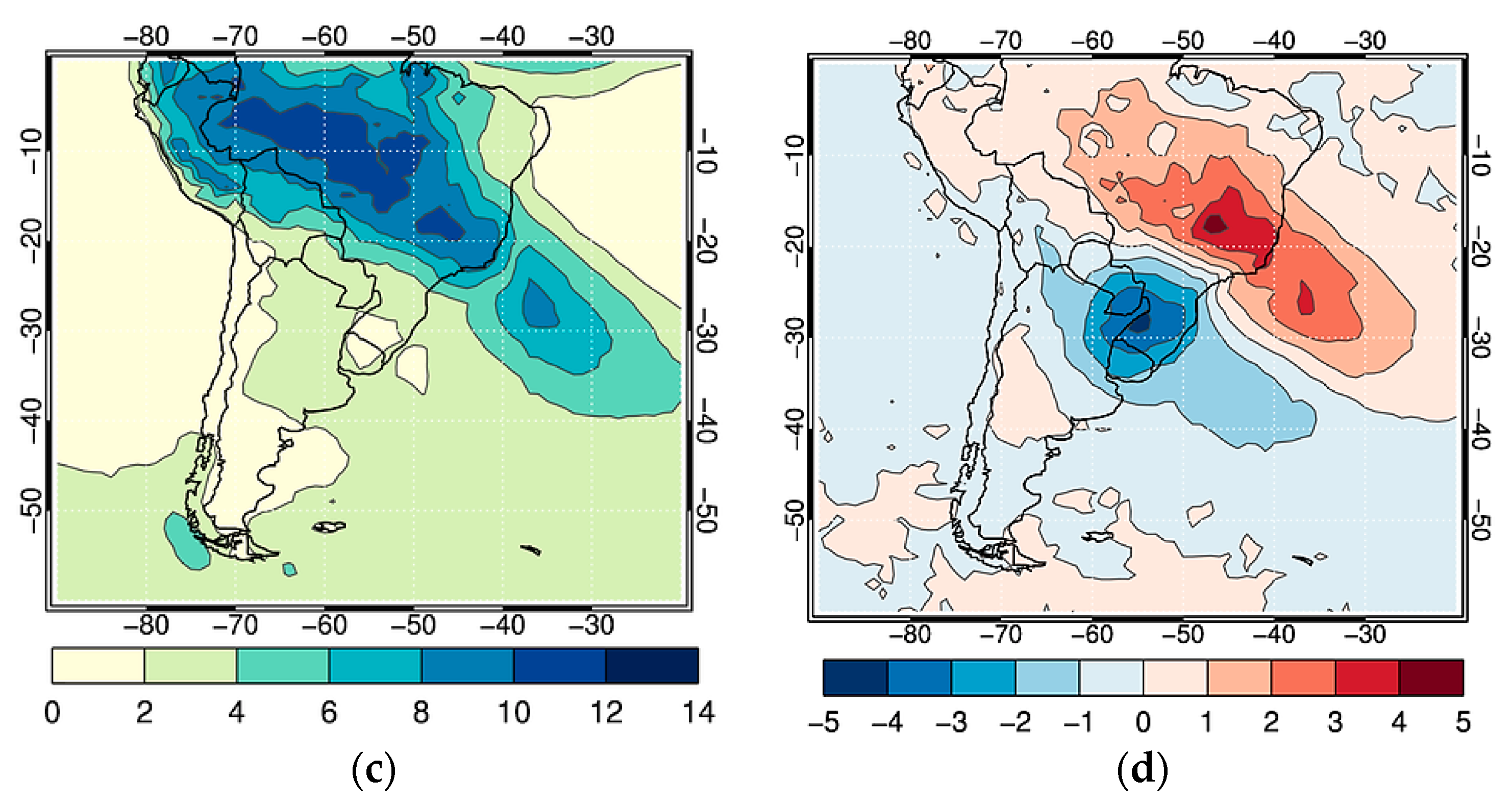
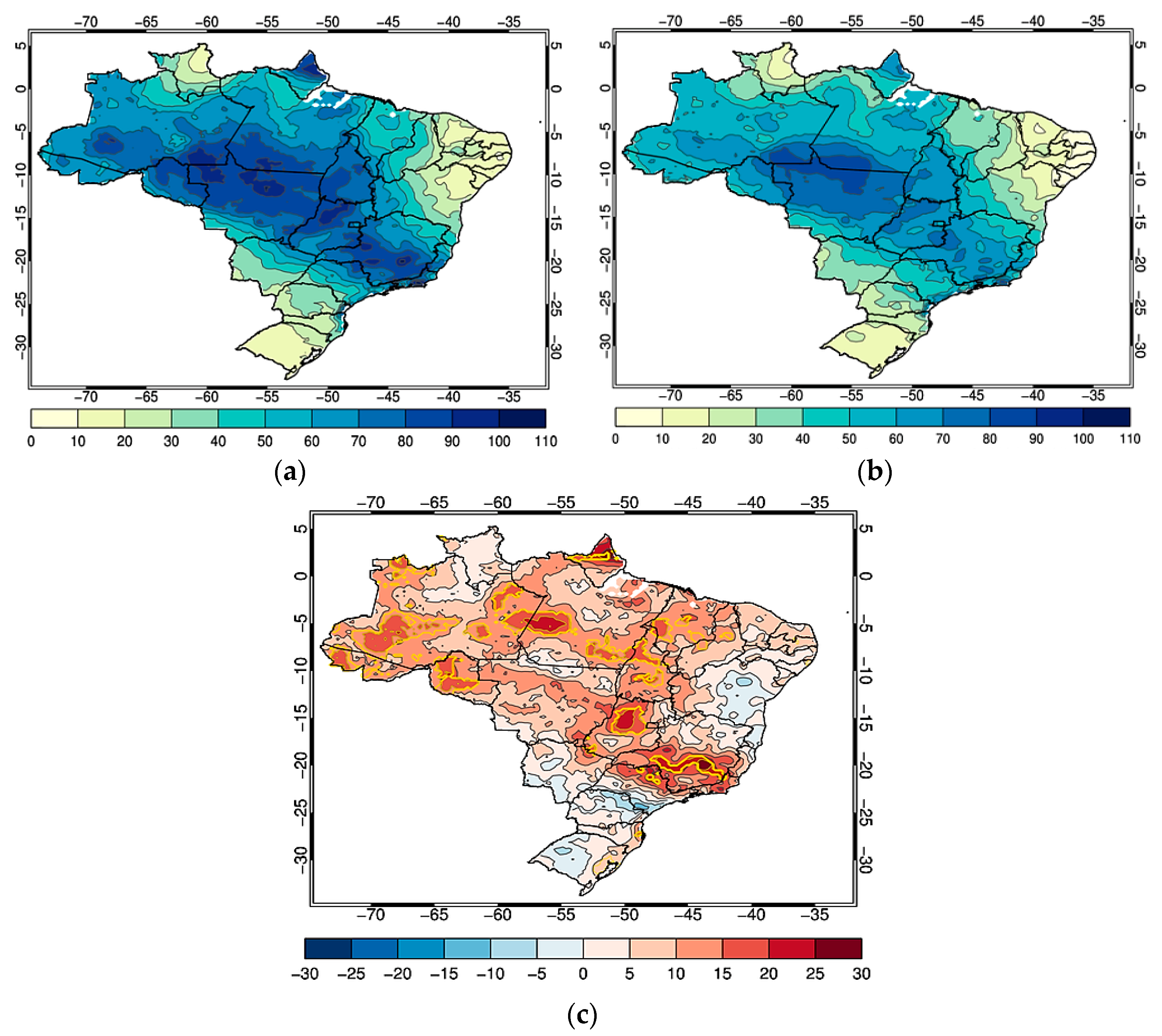
The average daily precipitation in the SACZ events (Figure 1a) clearly highlighted the characteristic of this phenomenon: northwest-southeast diagonal orientation of precipitation, with values up to 14 mm/day. Meanwhile, very low values of precipitation (below 2 mm/day) were observed in the extreme south of Brazil and in the eastern of the Northeast region. Figure 1b shows the highest values of difference over the SACZ region, especially in the southeast region, where the daily precipitation of the SACZ is greater than the daily precipitation of the summer. Figure 1c also showed the highest values of precipitation (up to 12 mm/day) in climatological SACZ region and in the adjacent ocean. Figure 1d shows the largest positive differences (up to +4 mm/day) on the SACZ region, also extending to the Atlantic Ocean.
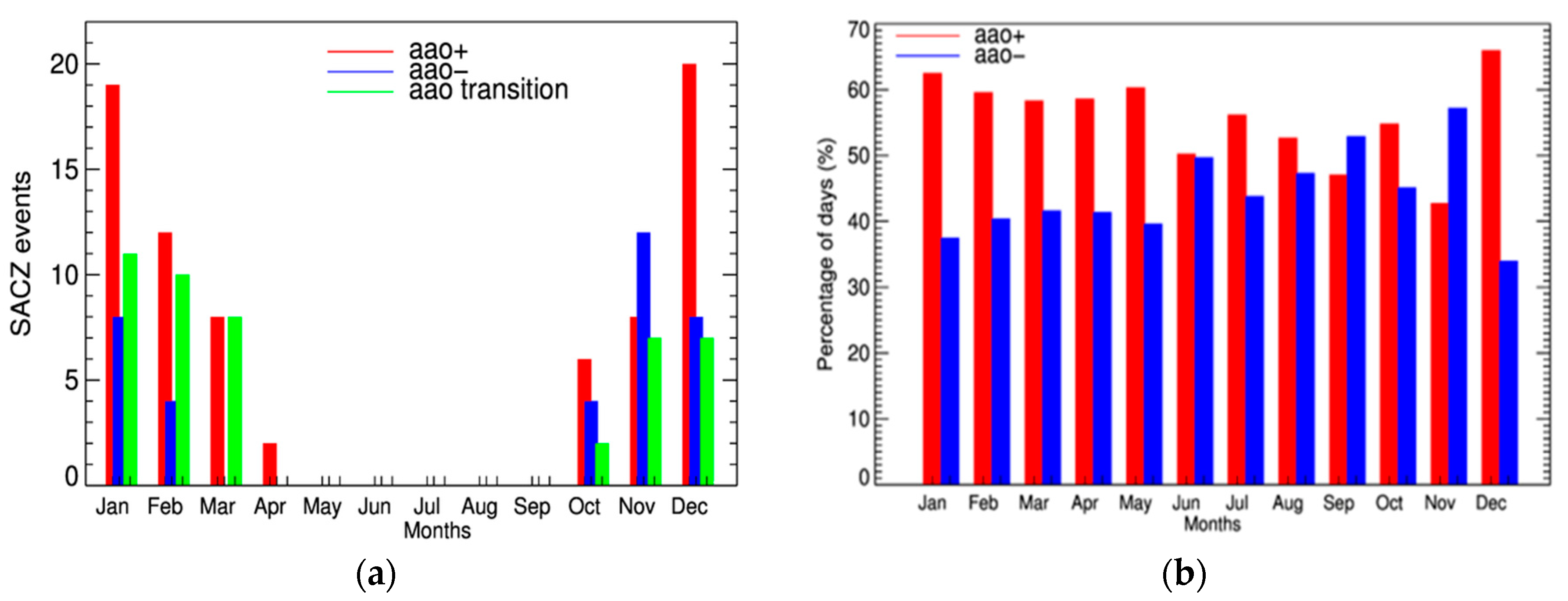
Approximately 65% of SACZ events occurred in AAO+ and approximately 35% in AAO−, indicating that SACZ events were more frequent in AAO+ due to the fact that the AAO+ is much longer than the AAO−, especially in DJFM (according to Figure 2). Approximately 28% of the SACZ events occurred in AAO transition periods.
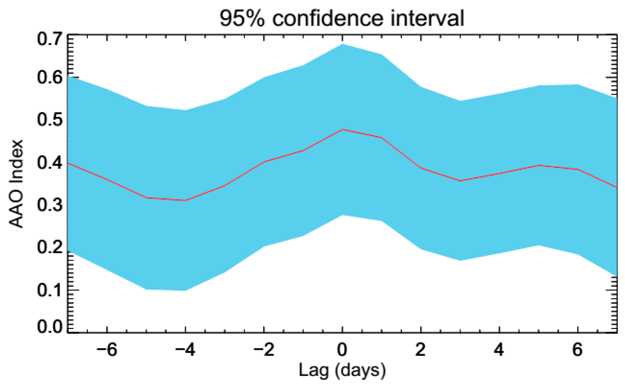
Figure 3 shows the temporal variation of the average daily AAO index over a previous week (lag = −7 days) up to a week after (lag = +7 days) at the beginning of SACZ events (lag = 0). Although there are negative AAO index values in some SACZ events (35%), the AAO+ is dominant in the SACZ events (65%), and therefore, when the mean index of the events was calculated, only positive values of AAO remained (Figure 3). It is also important to note that approximately four days before the beginning of an SACZ (lag = −4), the AAO index shows a growth, reaching its maximum at lag = 0 (beginning of the SACZ) and thereafter tends to decrease, reaching a minimum value in lag = +3. This AAO behavior can be used as a precursor to SACZ events, along with the other known characteristics of the phenomenon.
Figure 4 illustrates the boxplot of the persistence of SACZ events in each AAO phase. The maximum persistence in the SACZ events in AAO− was 7 days (upper whisker), and the median persistence was 6 days. In the SACZ events that occurred in AAO+, the maximum persistence was 12 days (upper whisker), and the median was 6 days. The outliers in AAO+ (AAO−) indicate that SACZ events have persistence longer than 12 days (7 days). Therefore, SACZ events tend to be more persistent and their variability is greater in AAO+.
The precipitation variability in the AAO phases indicates higher accumulated values on the climatological position of the SACZ in AAO+ (Figure 5a) than in AAO− (Figure 5b). The results obtained in Figure 5a are in agreement with those observed in previous studies (e.g., [13,14]) and alongside Figure 1. Over northeastern and southern Brazil, lower values of precipitation (below 20 mm/event) were observed associated with the SACZ (Figure 5a,b), according to studies of Cunningham and Cavalcanti [22], Nogués-Paegle and Mo [5] and Nogués-Paegle et al. [23]. Figure 5c shows the difference in mean accumulated precipitation (mm/event) between AAO+ and AAO-. It was observed that precipitation was higher (up to 30 mm/event) in the SACZ region in AAO+ than in AAO−, especially in the southeast region of Brazil.
A greater variability of the precipitation (standard deviation up to 90 mm/event) in AAO+ (Figure 6a) stands out than that in AAO− (Figure 6b), mainly in the Brazilian southeast. A lower variability of precipitation (less than 30 mm/event) in the south and northeast regions of Brazil was associated with SACZ events.
As can be observed in Figure 4, in addition to the SACZ persistence being lower in AAO− than in AAO+, resulting in lower values of accumulated precipitation (Figure 5), it has less variability in AAO− than in AAO+ (Figure 4). Thus, the accumulated precipitation variability between SACZ events in each phase of the AAO (Figure 6) tends to follow the persistence variability of the events (Figure 4).
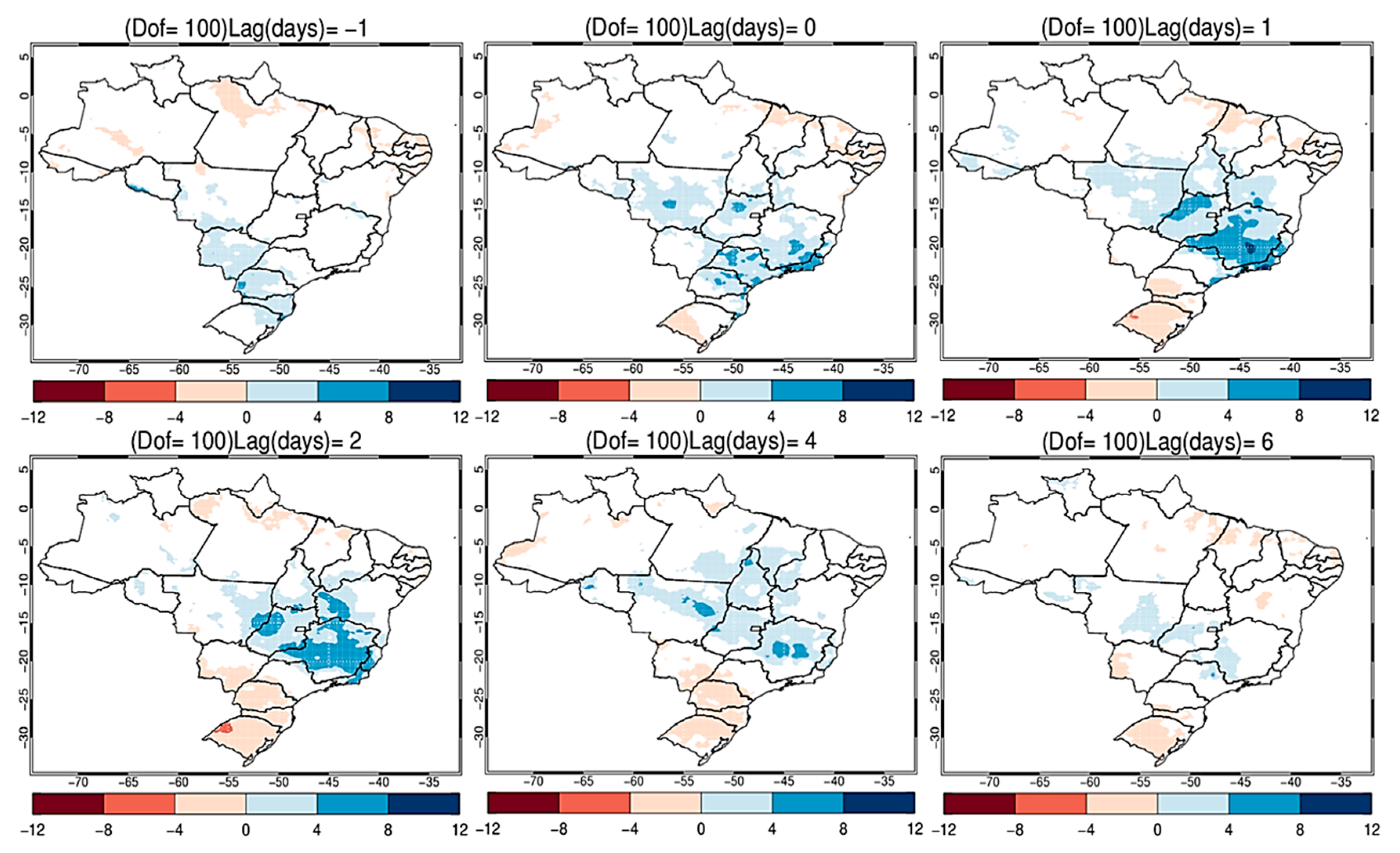
Figure 7 and Figure 8 show the lag composite of daily precipitation anomalies (mm) from days before (lag = −1) to days later (lag = +6) at the beginning of SACZ events (lag = 0) for AAO+ (Figure 7) and AAO− (Figure 8). In AAO+ (Figure 7), one day before the event (lag = −1), a range of positive anomalies appears in southern Brazil. From lag = 1, positive precipitation anomalies cover the entire climatological region of the SACZ (reaching up to +12mm/day in lag = 1), and they practically disappear in lag = 6. It is also noted that, from lag = 1 to lag = 6, negative precipitation anomalies appear throughout the southern region of Brazil, in agreement with previous studies (e.g., [5,22]).
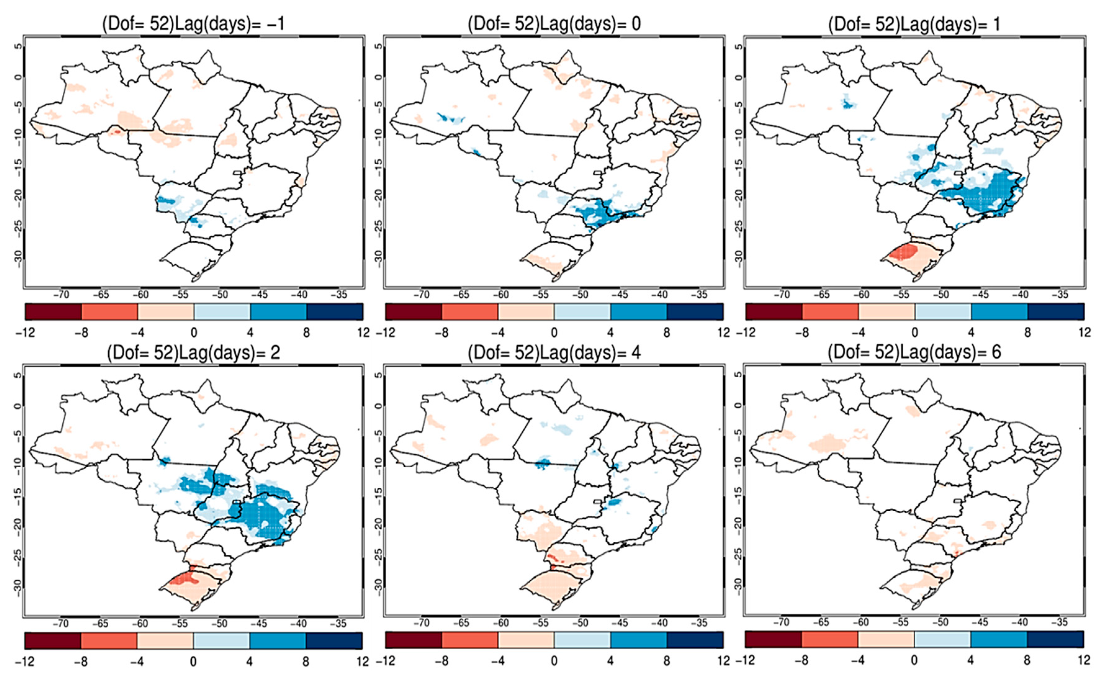
In AAO− (Figure 8), positive precipitation anomalies arise in the lag = 0 only in southeastern Brazil; they extend to the other regions of the SACZ until lag = 2 (up to +8 mm/day) and they disappear in the later lags. The negative precipitation anomalies in the south of Brazil appear in the lag = 1 until the lag = 4. In AAO− this dipole pattern of positive anomalies in the southeast and negative anomalies in the south of the Brazil practically disappears in the lag = 4 and lag = 6, whereas in AAO+ (Figure 7) it is still observed in these lags.
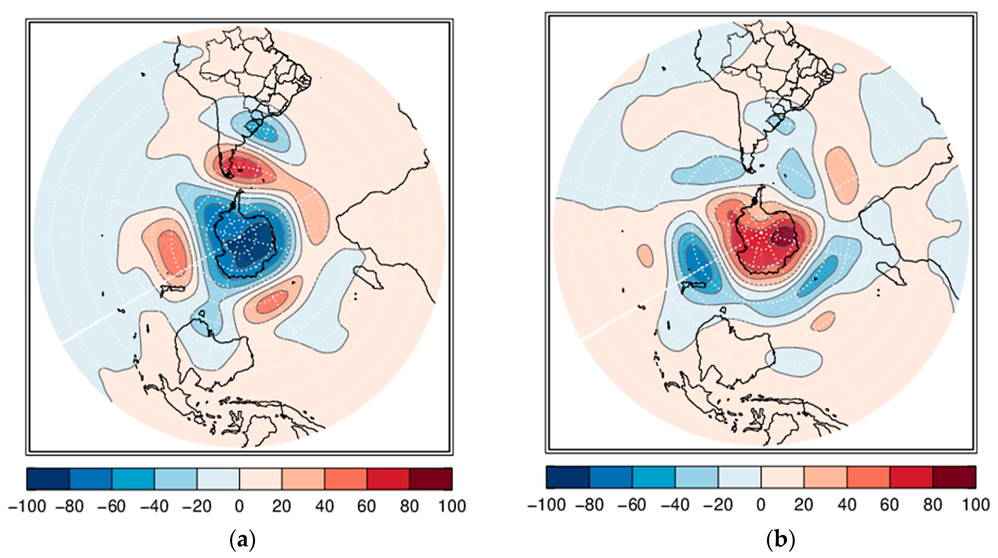
Figure 9 shows the composite of H700 anomalies at the beginning of SACZ events (lag = 0) for AAO+ (Figure 9a) and for AAO− (Figure 9b). This period was the one that best represented the AAO signature, with zonally symmetric anomalies between 40° S and 50° S and evidencing the two phases of this oscillation. It can be observed that in both phases, there is the establishment of negative anomalies in the climatological region of the SACZ, which are subtly more intense in southeastern Brazil.
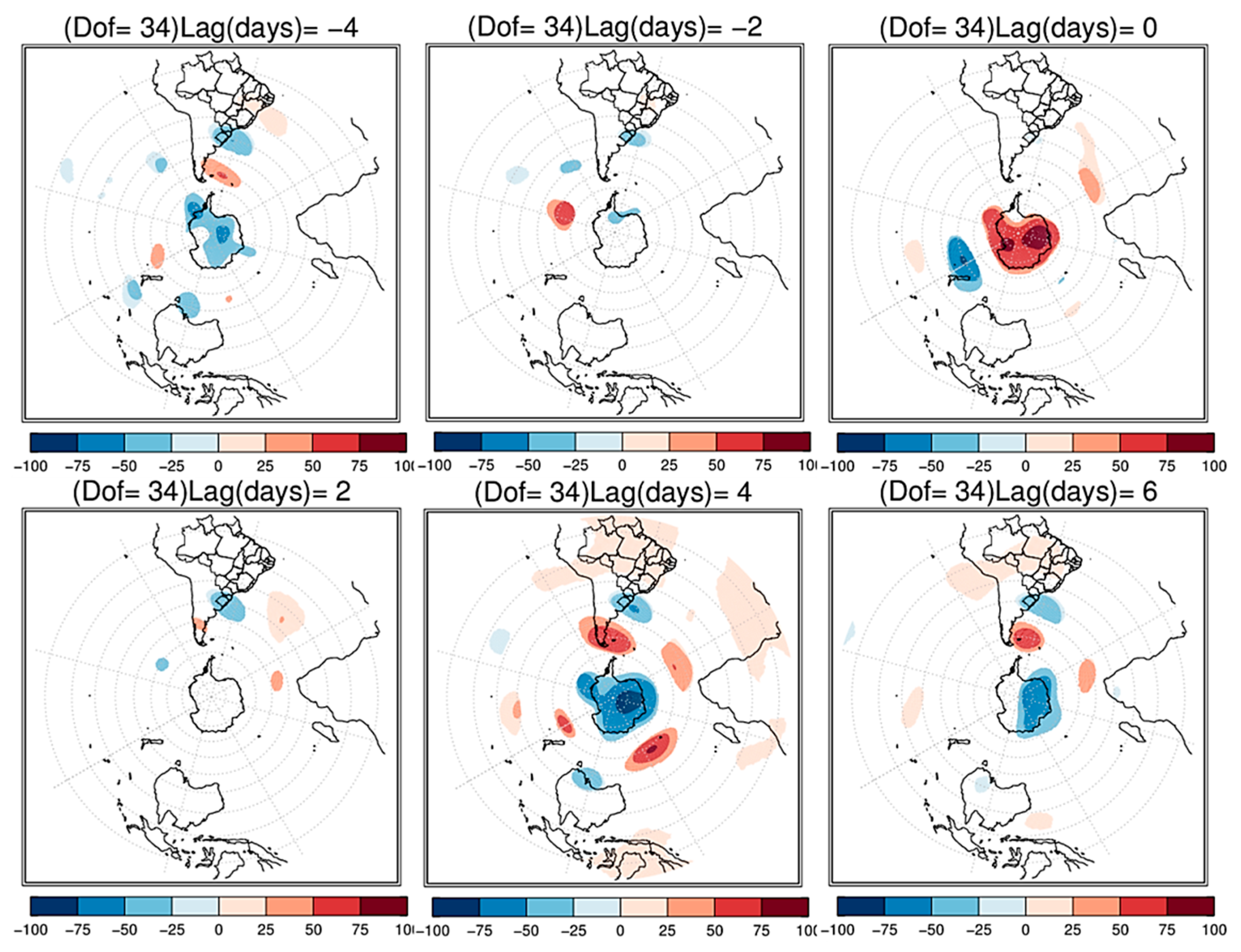
More intense positive H700 anomalies (up to +45 m) in AAO+ are observed over the circumpolar region at lag = 0, weakening up to lag = +6 days (Figure 10). Beginning from lag = −2, negative anomalies appear on the Antarctic continent, which become more intense (up to −60 m) in lag = 0. It can also be observed that in lag = −4 days, negative anomalies appear oriented in the northwest-southeast direction in South America, extending to the Atlantic Ocean, which become more extensive from lag = +2 days, suggesting a cyclonic circulation associated with upward movement at low levels (not shown). The H700 anomalies are somewhat different in AAO−: negative anomalies are distributed homogeneously over Brazil, from lag = −4 days, while the most significant positive anomalies (up to +60 m) appear only in lag = 0 over Antarctica (Figure 11).
A meridional wave train in H200 is observed throughout South America during the beginning of SACZ events, mainly in AAO+ (Figure 12a).
There is a diagonal band (NW/SE) of positive H200 anomalies displaced to the north of the climatological position of the SACZ and extending to the Atlantic Ocean in AAO+ (Figure 13), while in AAO−, this range is not well defined (Figure 14). In addition, negative anomalies are also observed over the southern region of Brazil in both phases of AAO. On the Antarctic continent, negative anomalies up to −100 m (lag = 0) appear in AAO+ (Figure 13), weakening from lag = +4 days; in AAO− (Figure 14), a signal inversion occurs, with intense positive anomalies only in lag = 0 (up to +100 m) and later, in lag = 4, these anomalies become negative and intense (up to −100 m). It is also important to note that H200 anomalies are persistent in South America in AAO+ for at least six days (Figure 13). This result suggests that the wave train in South America associated with SACZ events in AAO+ tends to be semi-stationary, which would explain the higher persistence of SACZ events in AAO+ than in AAO−.
Comparing the H700 (Figure 10 and Figure 11) and H200 anomalies (Figure 13 and Figure 14) in high latitudes, a vertical structure of the equivalent barotropic wave is observed in both AAO phases, whereas in SACZ region the wave train seems to be baroclinic.
H200 composites were recalculated using the same number of SACZ events in both phases of AAO and all with the same persistence (not shown). It was noted that the anomalies in AAO+ represented very well the AAO+ signature in events, whereas in AAO− there was no sign of anomalies about South America. That is, we still perceive more clearly the influence of AAO+ on these events than the AAO−.
Comparing the results at high and low levels, an equivalent barotropic structure between 40° S and 50° S can be verified, while the southern wave train observed on the South American continent has a more baroclinic characteristic that can be associated with transient frontal systems. During the summer, the frontal systems that advance towards the southeast region of Brazil can associate with the SACZ, intensifying it or even triggering an SACZ event [24,25,26,27].
Tropical-Extratropical Interaction in SACZ Events on the Intraseasonal Timescale
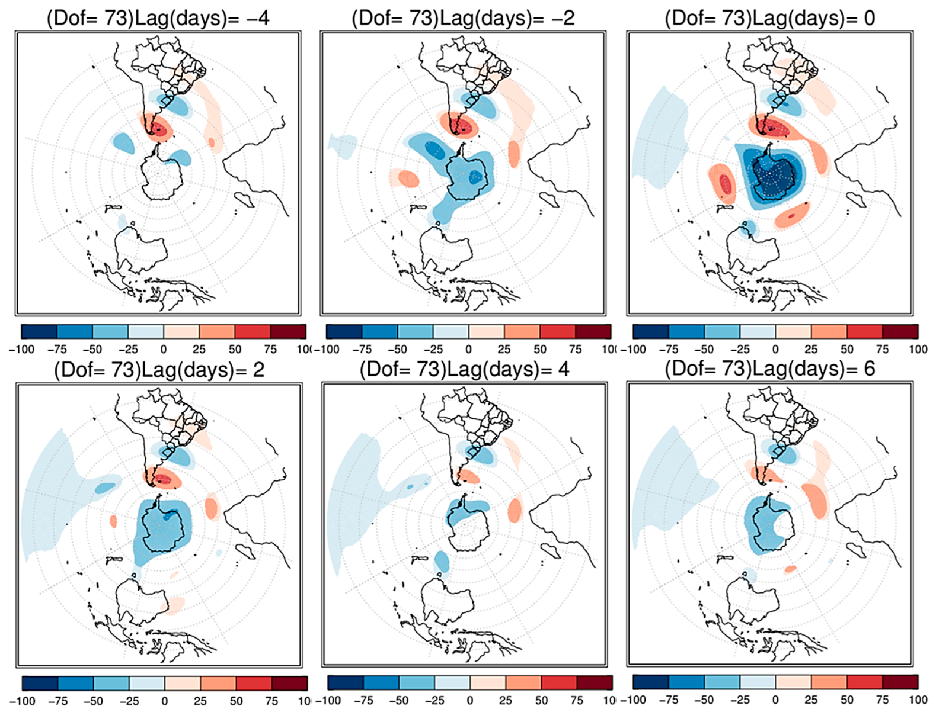
The next figures show the lag composite of intraseasonal anomalies of U200 in AAO+ (Figure 15) and AAO− (Figure 16). In AAO+, six days before the start of events (lag = ‒6) it is observed a robust wave train that moves from South Pacific Ocean to the South American continent (Figure 15). This meridional wave pattern is similar to the Pacific-South America (PSA) pattern [28,29]. A teleconnection mechanism between extratropics and SACZ region is evident in AAO+, through intensification of polar and subtropical jets, in days preceding SACZ (Figure 15). In AAO−, the wave train is not so evident and there is no clear signal of teleconnection between extratropics and SACZ (Figure 16). In addition, the anomalies on South America have a displacement to the South Atlantic Ocean, suggesting a possible mechanism for oceanic SACZ.
Carvalho et al. [30] investigated teleconnection patterns in U200 daily anomalies and also observed two symmetric zonal characteristics in ~45° S and ~60° S, which appear to be related to subtropical and polar jets, and that anomalies at high latitudes are weaker at AAO−, i.e., the weaker polar jet in this phase.
4. Conclusions
The goal of this study was to analyze the role of AAO phases in the statistical properties of SACZ events (frequency, persistence and intensity) and to analyze the vertical structure of atmospheric circulation during these events.
SACZ events were more persistent, intense (according to the accumulated precipitation) and frequent in AAO+, due to the fact that the AAO+ is much longer than the AAO−. In this case, a semi-stationary anticyclonic circulation in high and low levels of the troposphere was observed over the southern extreme of South America. The AAO+ better represented the precipitation signal associated with the SACZ, and the greater variability of this precipitation occurred in the southeast region of Brazil.
The dipole pattern of negative daily precipitation anomalies in the southern region of Brazil and positive anomalies on the SACZ region, in both phases of the AAO, coincides with previous studies. This signal is evident from the beginning of events (lag = 0) and lasts for at least up to four days (lag = 4), though, it is better defined and more comprehensive on the SACZ in the AAO+.
In relation to atmospheric circulation at low levels, a pattern was observed in both AAO+ and AAO− with negative anomalies of H700 in most of Brazil, including in the climatological position of the SACZ, indicating a cyclonic circulation. The most intense negative anomalies (up to −60 m) are seen in AAO+ on Antarctica (lag = 0). Positive anomalies of H700 were observed in AAO+ in southern South America, from lag = −4 to lag = 2, suggesting an anticyclonic circulation in that region. Nonetheless, the most intense positive anomalies (up to +60 m) are seen on Antarctica (lag = 0), but at AAO−.
In high levels of the troposphere, a dipole pattern appears with negative anomalies of H200 in the south of Brazil in AAO+, suggesting a cyclonic circulation, and an extensive range of H200 positive anomalies are displaced to the north of the climatological position of the SACZ, suggesting an anticyclonic circulation in this region. In AAO−, this pattern is seen less intensely throughout the events and for the most part is restricted on the continent.
Therefore, comparing the H700 and H200 anomalies, the region of high latitudes showed an equivalent barotropic structure, whereas in the SACZ region the southern wave train seems to be a baroclinic configuration, with amplitudes changing substantially with height.
The intraseasonal anomalies of U200 in the SACZ events showed an intense teleconnection pattern between the extratropics and the SACZ region in AAO+, associated with the intensification of the polar jet, whereas in AAO− this configuration was not so evident. In addition, the anomalies were more confined in the subtropical region and shifted to the South Atlantic Ocean in AAO−, suggesting a possible mechanism associated with the events of oceanic SACZ. However, other studies should be performed to evaluate the relationship between AAO phases and SACZ types.
The results found in this study indicated a strong modulation of the extratropical forcing in SACZ events associated with the AAO, which could be used as a precursor of the phenomenon because the AAO index had a substantial increase approximately four days before the beginning of SACZ events.
Author Contributions
Conceptualization, F.V.R., N.T.B., S.E.T.F. and T.C.R.; Formal analysis, F.V.R.; Methodology, F.V.R. and N.T.B.; Software, F.V.R. and T.C.R.; Supervision, N.T.B.; Visualization, F.V.R.; Writing–Original draft, F.V.R.; Writing–Review & editing, N.T.B. and S.E.T.F.
Acknowledgments
To CAPES for masters and PhD scholarships; Alexandre C. Xavier for the precipitation data; the ECMWF for the reanalysis data and the ANEEL R&D project developed in partnership between UTE Pecém II, UTE Parnaíba I, Parnaíba II and III Geração de Energia SA and the Federal University of Santa Maria-UFSM. Nathalie T. Boiaski thanks FAPERGS for funding research project no. 17/2551-0000821-9. Simone Ferraz thanks CNPq for the scholarship 304970/2015-8. We thank the anonymous reviewers for providing insightful comments and constructive suggestions to revise this article.
Conflicts of Interest
The authors declare no conflicts of interest.
Appendix A

Table A1.
Dates of SACZ events between 1992 and 2015.
| Initial Day | Final Day | Persistence |
|---|---|---|
| 12/01/1992 | 12/05/1992 | 5 |
| 01/09/1993 | 01/13/1993 | 5 |
| 02/02/1993 | 02/06/1993 | 5 |
| 02/09/1993 | 02/16/1993 | 8 |
| 02/22/1993 | 02/27/1993 | 6 |
| 12/18/1993 | 12/24/1993 | 7 |
| 12/27/1993 | 12/31/1993 | 5 |
| 01/01/1994 | 01/07/1994 | 7 |
| 01/09/1994 | 01/14/1994 | 6 |
| 12/15/1994 | 12/18/1994 | 4 |
| 01/26/1995 | 01/31/1995 | 6 |
| 02/01/1995 | 02/21/1995 | 21 |
| 12/05/1995 | 12/10/1995 | 6 |
| 12/13/1995 | 12/16/1995 | 4 |
| 12/26/1995 | 12/31/1995 | 6 |
| 01/01/1996 | 01/11/1996 | 11 |
| 01/16/1996 | 01/21/1996 | 6 |
| 02/03/1996 | 02/25/1996 | 23 |
| 03/01/1996 | 03/11/1996 | 11 |
| 01/02/1997 | 01/08/1997 | 7 |
| 01/20/1997 | 01/29/1997 | 10 |
| 03/01/1997 | 03/05/1997 | 5 |
| 03/17/1997 | 03/23/1997 | 7 |
| 11/14/1997 | 11/19/1997 | 6 |
| 02/12/1998 | 02/16/1998 | 5 |
| 11/20/1998 | 11/25/1998 | 6 |
| 01/06/1999 | 01/18/1999 | 13 |
| 10/24/1999 | 11/03/1999 | 11 |
| 11/17/1999 | 11/25/1999 | 9 |
| 12/08/1999 | 12/14/1999 | 7 |
| 12/16/1999 | 12/20/1999 | 5 |
| 01/01/2000 | 01/08/2000 | 8 |
| 01/21/2000 | 01/24/2000 | 4 |
| 02/06/2000 | 02/13/2000 | 8 |
| 12/01/2000 | 12/08/2000 | 8 |
| 12/17/2000 | 12/22/2000 | 6 |
| 01/01/2001 | 01/04/2001 | 4 |
| 11/01/2001 | 11/06/2001 | 6 |
| 11/16/2001 | 11/21/2001 | 6 |
| 12/17/2001 | 12/21/2001 | 5 |
| 12/24/2001 | 12/28/2001 | 5 |
| 02/04/2002 | 02/07/2002 | 4 |
| 02/16/2002 | 02/24/2002 | 9 |
| 12/10/2002 | 12/16/2002 | 7 |
| 12/27/2002 | 01/07/2003 | 12 |
| 01/13/2003 | 01/19/2003 | 7 |
| 01/25/2003 | 02/01/2003 | 8 |
| 01/02/2004 | 01/06/2004 | 5 |
| 01/10/2004 | 01/20/2004 | 11 |
| 01/25/2004 | 01/29/2004 | 5 |
| 02/07/2004 | 02/11/2004 | 5 |
| 02/20/2004 | 02/24/2004 | 5 |
| 11/20/2004 | 11/25/2004 | 6 |
| 12/09/2004 | 12/14/2004 | 6 |
| 12/21/2004 | 12/25/2004 | 5 |
| 01/17/2005 | 01/21/2005 | 5 |
| 02/13/2005 | 02/22/2005 | 10 |
| 03/01/2005 | 03/07/2005 | 7 |
| 03/15/2005 | 03/20/2005 | 6 |
| 11/10/2005 | 11/15/2005 | 6 |
| 11/17/2005 | 11/21/2005 | 5 |
| 11/24/2005 | 11/28/2005 | 5 |
| 12/11/2005 | 12/16/2005 | 6 |
| 12/24/2005 | 12/29/2005 | 6 |
| 01/01/2006 | 01/08/2006 | 8 |
| 01/27/2006 | 02/02/2006 | 7 |
| 02/09/2006 | 02/13/2006 | 5 |
| 03/07/2006 | 03/16/2006 | 10 |
| 10/17/2006 | 10/20/2006 | 4 |
| 11/10/2006 | 11/14/2006 | 5 |
| 11/26/2006 | 12/02/2006 | 7 |
| 12/07/2006 | 12/16/2006 | 10 |
| 12/27/2006 | 01/16/2007 | 21 |
| 01/22/2007 | 01/27/2007 | 6 |
| 01/30/2007 | 02/09/2007 | 11 |
| 02/12/2007 | 02/17/2007 | 6 |
| 03/19/2007 | 03/23/2007 | 5 |
| 10/22/2007 | 10/26/2007 | 5 |
| 11/04/2007 | 11/07/2007 | 4 |
| 11/27/2007 | 12/02/2007 | 6 |
| 12/19/2007 | 12/24/2007 | 6 |
| 01/06/2008 | 01/09/2008 | 4 |
| 01/20/2008 | 01/24/2008 | 5 |
| 01/30/2008 | 02/08/2008 | 10 |
| 02/22/2008 | 02/25/2008 | 4 |
| 02/26/2008 | 02/29/2008 | 4 |
| 03/03/2008 | 03/08/2008 | 6 |
| 03/12/2008 | 03/17/2008 | 6 |
| 10/18/2008 | 10/21/2008 | 4 |
| 11/07/2008 | 11/11/2008 | 5 |
| 11/13/2008 | 11/24/2008 | 12 |
| 11/27/2008 | 12/01/2008 | 5 |
| 12/03/2008 | 12/07/2008 | 5 |
| 12/12/2008 | 12/20/2008 | 9 |
| 12/25/2008 | 12/28/2008 | 4 |
| 01/04/2009 | 01/08/2009 | 5 |
| 01/20/2009 | 01/24/2009 | 5 |
| 02/12/2009 | 02/16/2009 | 5 |
| 03/13/2009 | 03/16/2009 | 4 |
| 03/22/2009 | 04/02/2009 | 12 |
| 04/08/2009 | 04/12/2009 | 5 |
| 10/08/2009 | 10/11/2009 | 4 |
| 10/21/2009 | 10/24/2009 | 4 |
| 10/27/2009 | 11/03/2009 | 8 |
| 12/04/2009 | 12/09/2009 | 6 |
| 12/12/2009 | 12/15/2009 | 4 |
| 01/20/2010 | 01/23/2010 | 4 |
| 02/28/2010 | 03/04/2010 | 5 |
| 03/06/2010 | 03/12/2010 | 7 |
| 04/07/2010 | 04/12/2010 | 6 |
| 10/31/2010 | 11/04/2010 | 5 |
| 11/06/2010 | 11/12/2010 | 7 |
| 11/24/2010 | 11/28/2010 | 5 |
| 11/30/2010 | 12/06/2010 | 7 |
| 12/13/2010 | 12/17/2010 | 5 |
| 12/27/2010 | 12/31/2010 | 5 |
| 01/01/2011 | 01/07/2011 | 7 |
| 01/11/2011 | 01/16/2011 | 6 |
| 01/18/2011 | 01/21/2011 | 4 |
| 02/09/2011 | 02/16/2011 | 8 |
| 02/28/2011 | 03/09/2011 | 10 |
| 03/10/2011 | 03/18/2011 | 9 |
| 10/17/2011 | 10/21/2011 | 5 |
| 10/31/2011 | 11/04/2011 | 5 |
| 11/22/2011 | 11/29/2011 | 8 |
| 12/01/2011 | 12/04/2011 | 4 |
| 12/14/2011 | 12/21/2011 | 8 |
| 12/25/2011 | 12/30/2011 | 6 |
| 01/01/2012 | 01/08/2012 | 8 |
| 01/14/2012 | 01/20/2012 | 7 |
| 01/26/2012 | 01/30/2012 | 5 |
| 02/11/2012 | 02/14/2012 | 4 |
| 03/16/2012 | 03/21/2012 | 6 |
| 11/04/2012 | 11/08/2012 | 5 |
| 11/14/2012 | 11/22/2012 | 9 |
| 11/25/2012 | 11/28/2012 | 4 |
| 12/14/2012 | 12/17/2012 | 4 |
| 01/09/2013 | 01/14/2013 | 6 |
| 01/19/2013 | 01/23/2013 | 5 |
| 01/26/2013 | 01/31/2013 | 6 |
| 02/03/2013 | 02/06/2013 | 4 |
| 02/07/2013 | 02/14/2013 | 8 |
| 03/15/2013 | 03/19/2013 | 5 |
| 03/21/2013 | 03/31/2013 | 11 |
| 10/04/2013 | 10/09/2013 | 6 |
| 10/17/2013 | 10/20/2013 | 4 |
| 11/04/2013 | 11/08/2013 | 5 |
| 11/22/2013 | 11/26/2013 | 5 |
| 12/11/2013 | 12/26/2013 | 16 |
| 01/17/2014 | 01/21/2014 | 5 |
| 02/15/2014 | 02/18/2014 | 4 |
| 11/14/2014 | 11/19/2014 | 6 |
| 11/26/2014 | 11/29/2014 | 4 |
| 12/22/2014 | 12/25/2014 | 4 |
| 02/04/2015 | 02/08/2015 | 5 |
| 02/15/2015 | 02/18/2015 | 4 |
References
- Quadro, M.F.L. Estudo de episódios de Zona de Convergência do Atlântico Sul (ZCAS) sobre a América do Sul. Master’s Thesis, Instituto Nacional de Pesquisas Espaciais, São José dos Campos-SP, Brazil, 1994. [Google Scholar]
- Satyamurty, P.; Mattos, L.F. Climatological lower tropospheric frontogenesis in the midlatitudes due to horizontal deformation and divergence. Mon. Weather Rev. 1989, 117, 119–139. [Google Scholar] [CrossRef]
- Kodama, Y. Large-scale common features of subtropical precipitation zones (the Baiu Frontal Zone, the SPCZ, and the SACZ). Part I: characteristics of subtropical frontal zones. J. Meteor. Soc. Jpn. 1992, 70, 813–835. [Google Scholar] [CrossRef]
- Wiel, K.V.D.; Matthews, A.J.; Stevens, D.P.; Joshi, M.M. A dynamical framework for the origin of the diagonal South Pacific and South Atlantic Convergence Zones. Q. J. R. Meteorol. Soc. 2015, 141, 1997–2010. [Google Scholar] [CrossRef] [Green Version]
- Nogués-Paegle, J.; Mo, K.C. Alternating wet and dry conditions over South America during summer. Mon. Weather Rev. 1997, 125, 279–291. [Google Scholar] [CrossRef]
- Tomaziello, A.C.N. Influências da temperatura da superfície do mar e da umidade do solo na precipitação associada à Zona de Convergência do Atlântico Sul. Master’s Thesis, Universidade de São Paulo, São Paulo, Brazil, 2010. [Google Scholar] [Green Version]
- Carvalho, L.M.V.; Jones, C.; Liebmann, B. The South Atlantic Convergence Zone: Intensity, Form, Persistence, and Relationships with Intraseasonal to Interannual Activity and Extreme Rainfall. J. Clim. 2004, 17, 88–108. [Google Scholar] [CrossRef] [Green Version]
- Alvarez, M.S.; Vera, C.S.; Kiladis, G.N. MJO modulating the activity of the leading mode of intraseasonal variability in South America. Atmosphere 2017, 8, 232. [Google Scholar] [CrossRef]
- Gong, D.Y.; Wang, S.W. Definition of Antarctic oscillation index. Geophys. Res. Lett. 1999, 26, 459–462. [Google Scholar] [CrossRef]
- Thompson, D.W.J.; Wallace, J.M. Annular modes in the extratropical circulation. Part I: Month-to-Month Variability. J. Clim. 2000, 13, 1000–1016. [Google Scholar] [CrossRef]
- Mo, K.C. Relationships between low-frequency variability in the Southern Hemisphere and sea surface temperature anomalies. J. Clim. 2000, 13, 3599–3610. [Google Scholar] [CrossRef]
- Reboita, M.S.; Ambrizzi, T.; Da Rocha, R.P. Relationship between the Southern Annular Mode and Southern Hemisphere Atmospheric Systems. Revista Brasileira de Meteorologia 2009, 24, 48–55. [Google Scholar] [CrossRef]
- Silvestri, G.E.; Vera, C.S. Antarctic Oscillation signal on precipitation anomalies over southeastern South America. Geophys. Res. Lett. 2003, 30, 2115. [Google Scholar] [CrossRef]
- Vasconcellos, F.C.; Cavalcanti, I.F.A. Extreme Precipitation over Southeastern Brazil in the Austral Summer and Relations with the Southern Hemisphere Annular Mode. Atmos. Sci. Lett. 2010, 11, 21–26. [Google Scholar] [CrossRef]
- Climanálise. Boletim de Monitoramento e Análise Climática. Centro de Previsão de Tempo e Estudos Climáticos/Instituto Nacional de Meteorologia (CPTEC/INMET) 2013, 28, p. 47. Available online: https://climanalise.cptec.inpe.br/~rclimanl/boletim/ (accessed on 17 June 2018).
- Cerne, S.B.; Vera, C.S.; Liebmann, B. The nature of a heat wave in eastern Argentina occurring during SALLJEX. Mon. Weather Rev. 2007, 135, 1165–1174. [Google Scholar] [CrossRef]
- Cerne, S.B.; Vera, C.S. Influence of the intraseasonal variability on heat waves in subtropical South America. Clim. Dynam. 2011, 36, 2265–2277. [Google Scholar] [CrossRef]
- Xavier, A.C.; King, C.W.; Scanlon, B.R. Daily gridded meteorological variables in Brazil (1980–2013). Int. J. Climatol. 2016, 36, 2644–2659. [Google Scholar] [CrossRef]
- Xavier, A.C.; King, C.W.; Scanlon, B.R. An update of Xavier, King and Scanlon (2016) daily precipitation gridded data set for the Brazil. In Proceedings of the 18th Brazilian Symposium on Remote Sensing, Santos, São Paulo, Brazil, 2017; Available online: http://careyking.com/wp-content/uploads/2017/08/Xavier-et-al-2017-SBSR-Update-of-Brazil-precipitation-gridded-data-set.pdf (accessed on 17 June 2018).
- Huffman, G.J. Global precipitation at one-degree daily resolution from multisatellite observations. J. Hydrometeorol. 2001, 2, 36–50. [Google Scholar] [CrossRef]
- Dee, D.P. The ERA-Interim Archive, Version 2.0. ERA Report Series. 1. Technical Report. ECMWF 2011, p. 23. Available online: https://www.ecmwf.int/en/elibrary/8174-era-interim-archive-version-20 (accessed on 17 June 2018).
- Cunningham, C.A.C.; Cavalcanti, I.F.A. Intraseasonal modes of variability affecting the South Atlantic Convergence Zone. Int. J. Climatol. 2006, 26, 1165–1180. [Google Scholar] [CrossRef] [Green Version]
- Nogués-Paegle, J.; Byerle, L.A.; Mo, K.C. Intraseasonal modulation of South American summer precipitation. Mon. Weather Rev. 2000, 128, 837–850. [Google Scholar] [CrossRef]
- Oliveira, A.S. Interações entre sistemas frontais na América do Sul e convecção da Amazônia. Master’s Thesis, Instituto Nacional de Pesquisas Espaciais, São José dos Campos, Brazil, 1986. [Google Scholar]
- Scheuer, P.R. Sistemas frontais associados a episódios de Zona de Convergência do Atlântico Sul. Undergraduate Thesis, Universidade Federal de Santa Catarina, Florianópolis, Brazil, 2017. [Google Scholar]
- Satyamurty, A.B.; Mattos, L.F.; Nobre, C.A.; Silva Dias, P.L. Tropics—South America. In Meteorology of the Southern Hemisphere; Kauly, D.J., Vicent, D.G., Eds.; American Meteorological Society: Boston, MA, USA, 1998; pp. 119–139. [Google Scholar]
- Ferreira, N.J.; Ramírez, M.V.; Gan, M.A. Vórtices ciclônicos de altos níveis que atuam na vizinhança do Nordeste do Brasil. In Tempo e Clima no Brasil; Oficina de Textos: São Paulo, Brazil, 2009; p. 43. [Google Scholar]
- Mo, K.C.; Ghil, M. Statistics and dynamics of persistent anomalies. J. Atmos. Sci. 1987, 44, 877–902. [Google Scholar] [CrossRef]
- Ghil, M.; Mo, K.C. Intraseasonal oscillations in the global atmosphere. Part II: Southern Hemisphere. J. Atmos. Sci. 1991, 48, 780–790. [Google Scholar] [CrossRef]
- Carvalho, L.M.V.; Jones, C.; Ambrizzi, T. Opposite phases of the Antarctic oscillation and relationships with intraseasonal to interannual activity in the tropics during the austral summer. J. Clim. 2005, 18, 702–718. [Google Scholar] [CrossRef]
Figure 1.
(a) Average daily precipitation (mm/day) in the SACZ events and (b) difference (in mm) between (a) and the average daily precipitation for October to March; (c) the same as (a) but for GPCP data and (d) the same as (b) but for GPCP data.
Figure 1.
(a) Average daily precipitation (mm/day) in the SACZ events and (b) difference (in mm) between (a) and the average daily precipitation for October to March; (c) the same as (a) but for GPCP data and (d) the same as (b) but for GPCP data.


Figure 2.
(a) Monthly frequency of the number of SACZ events in each phase of AAO and in AAO transition periods and (b) the percentage (%) of days in each phase of AAO, both for the period 1992–2015. The red bars are for AAO+, the blue bars for AAO− and green bars for AAO transition periods.
Figure 2.
(a) Monthly frequency of the number of SACZ events in each phase of AAO and in AAO transition periods and (b) the percentage (%) of days in each phase of AAO, both for the period 1992–2015. The red bars are for AAO+, the blue bars for AAO− and green bars for AAO transition periods.

Figure 3.
Average AAO index (red line) during the previous week (lag = −7 days) up to a week after (lag = +7 days) at the beginning of SACZ events (lag = 0). The blue shaded area is the 95% confidence interval, assuming normality.
Figure 3.
Average AAO index (red line) during the previous week (lag = −7 days) up to a week after (lag = +7 days) at the beginning of SACZ events (lag = 0). The blue shaded area is the 95% confidence interval, assuming normality.

Figure 4.
Boxplot of persistence (days) of SACZ events in AAO− and AAO+. The red circles represent the outliers, the box represents the interquartile range (IQ), the upper whisker is given by the upper quartile +1.5 × IQ, and the lower whisker is given by the lower quartile −1.5 × IQ.
Figure 4.
Boxplot of persistence (days) of SACZ events in AAO− and AAO+. The red circles represent the outliers, the box represents the interquartile range (IQ), the upper whisker is given by the upper quartile +1.5 × IQ, and the lower whisker is given by the lower quartile −1.5 × IQ.

Figure 5.
Composite of accumulated precipitation (mm/event) during SACZ events at (a) AAO+, (b) AAO−, and (c) difference between (a,b). Yellow outlines in bold indicate values that were statistically significant at the 5% level.
Figure 5.
Composite of accumulated precipitation (mm/event) during SACZ events at (a) AAO+, (b) AAO−, and (c) difference between (a,b). Yellow outlines in bold indicate values that were statistically significant at the 5% level.

Figure 6.
Mean standard deviation of accumulated precipitation (mm/event) in SACZ episodes (a) at AAO+ and (b) at AAO−.
Figure 6.
Mean standard deviation of accumulated precipitation (mm/event) in SACZ episodes (a) at AAO+ and (b) at AAO−.

Figure 7.
Lag composite of daily precipitation anomalies (mm/day) of SACZ events for AAO+. Shaded areas in blue (red) are for the positive (negative) values statistically significant at the 5% level, based on Student’s t-test. Dof is the degrees of freedom. The lags are indicated at the top of each figure.

Figure 8.
The same as Figure 7 but for AAO−.
Figure 8.
The same as Figure 7 but for AAO−.

Figure 9.
Composite of geopotential height anomalies (m) at 700 hPa during the beginning of SACZ events (lag = 0) in (a) AAO+ and (b) AAO−.
Figure 9.
Composite of geopotential height anomalies (m) at 700 hPa during the beginning of SACZ events (lag = 0) in (a) AAO+ and (b) AAO−.

Figure 10.
Lag composite of geopotential height anomalies (m) at 700 hPa during SACZ events at AAO+. Shaded areas in red (blue) are for the positive (negative) values statistically significant at the 5% level, based on Student’s t-test. Dof is the degrees of freedom.
Figure 10.
Lag composite of geopotential height anomalies (m) at 700 hPa during SACZ events at AAO+. Shaded areas in red (blue) are for the positive (negative) values statistically significant at the 5% level, based on Student’s t-test. Dof is the degrees of freedom.

Figure 11.
The same as Figure 10 but for AAO−.
Figure 11.
The same as Figure 10 but for AAO−.

Figure 12.
The same as Figure 9 but at 200 hPa.
Figure 12.
The same as Figure 9 but at 200 hPa.

Figure 13.
The same as Figure 10 but at 200 hPa.
Figure 13.
The same as Figure 10 but at 200 hPa.

Figure 14.
The same as Figure 13 but for AAO−.
Figure 14.
The same as Figure 13 but for AAO−.

Figure 15.
Lag composite of intraseasonal anomalies of the zonal wind (m/s) at 200 hPa during SACZ events at AAO+. Shaded areas in red (blue) are for the positive (negative) values statistically significant at the 5% level, based on Student’s t-test. Dof is the degrees of freedom.
Figure 15.
Lag composite of intraseasonal anomalies of the zonal wind (m/s) at 200 hPa during SACZ events at AAO+. Shaded areas in red (blue) are for the positive (negative) values statistically significant at the 5% level, based on Student’s t-test. Dof is the degrees of freedom.

Figure 16.
The same as Figure 15 but for AAO−.
Figure 16.
The same as Figure 15 but for AAO−.

© 2018 by the authors. Licensee MDPI, Basel, Switzerland. This article is an open access article distributed under the terms and conditions of the Creative Commons Attribution (CC BY) license (http://creativecommons.org/licenses/by/4.0/).
Share and Cite
MDPI and ACS Style
Rosso, F.V.; Boiaski, N.T.; Ferraz, S.E.T.; Robles, T.C. Influence of the Antarctic Oscillation on the South Atlantic Convergence Zone. Atmosphere 2018, 9, 431. https://doi.org/10.3390/atmos9110431
AMA Style
Rosso FV, Boiaski NT, Ferraz SET, Robles TC. Influence of the Antarctic Oscillation on the South Atlantic Convergence Zone. Atmosphere. 2018; 9(11):431. https://doi.org/10.3390/atmos9110431
Chicago/Turabian StyleRosso, Flávia Venturini, Nathalie Tissot Boiaski, Simone Erotildes Teleginski Ferraz, and Tiago Capello Robles. 2018. "Influence of the Antarctic Oscillation on the South Atlantic Convergence Zone" Atmosphere 9, no. 11: 431. https://doi.org/10.3390/atmos9110431
Note that from the first issue of 2016, this journal uses article numbers instead of page numbers. See further details here.