
Evaluation of InVEST’s Water Ecosystem Service Models in a Brazilian Subtropical Basin


Center for Water Resources and Environmental Studies, Sao Carlos School of Engineering, University of Sao Paulo, São Carlos 13566-590, SP, Brazil
*
Author to whom correspondence should be addressed.
Water 2022, 14(10), 1559; https://doi.org/10.3390/w14101559
Submission received: 26 February 2022
/
Revised: 4 May 2022
/
Accepted: 10 May 2022
/
Published: 12 May 2022
(This article belongs to the Section Ecohydrology)
Abstract
:The biophysical modeling of water ecosystem services is crucial to understanding their availability, vulnerabilities, and fluxes. Among the most popular models, the Integrated Valuation of Ecosystem Services and Trade-offs (InVEST) models stand out. While many studies have used them, few have assessed their performance. This study evaluates the performance of InVEST’s Seasonal Water Yield, Nutrient Delivery Ratio, and Sediment Delivery Ratio models in a subtropical basin in southeastern Brazil on temporal and spatial scales, using 39 years of streamflow data, 29 for total phosphorus and total nitrogen, and 19 for total suspended solids. Statistical indicators R2, PBIAS, and NSE, were also calculated. The performance of the models varied according to the type of simulated WES and analysis scales used, with the Seasonal Water Yield model demonstrating the best performance and effectively representing the spatial and temporal variability of the average annual streamflow. All models performed well in simulating long-term mean values when compared to observed data. While one should bear in mind the study’s limitations, the results indicate that the models perform well in terms of relative magnitude, although their application in studies involving water-resource management and decision making is limited.
1. Introduction
A water ecosystem services (WES)-based approach, incorporating an integrated analysis among multiple pressures, ecological statuses, and ecosystem services has been identified as an effective tool to plan and manage water resources, as it links environmental conservation with socioeconomic development [1]. Such an approach enables an assessment of how anthropic activities affect ecosystem composition and functioning, impacting WES, including water supply services for human use, irrigation, and energy generation, as well as regulation services associated with flood mitigation, erosion control, and water purification [2].
A pillar of this approach is biophysical modeling, which quantifies WES from mathematical equations in computational environments [3]. Biophysical models facilitate the understanding of ecohydrological processes in hydrographic basins and the assessment and forecasting of multiple pressures [1]. Well-calibrated, validated models have numerous applications in water management, such as quantifying the effects of land use and climate change [4,5,6], assessing flood risk [7], and designing and evaluating forest restoration programs [8,9,10,11], in addition to generating and transferring historical data for unmonitored basins, which is critical for hydrological studies [12]. Such applications can help formulate and evaluate environmental conservation policies that support sound decision making in water resource management and land-use planning [13].
Over the past few decades, free models to map ecosystem services have emerged [14,15,16], ranging from simple approaches based on land-use data or habitat-based proxies to complex models that quantify physical processes in ecosystems [3]. Traditional hydrological models such as the Soil and Water Assessment Tool (SWAT) [17], Variable Infiltration Capacity model [18], and the Regional Hydro-Ecological Simulation System [19] can be used to map and quantify WES. While they can accurately represent ecohydrological processes critical to a broad spectrum of ecosystem services, such as drinking water and recreation [1,20], their application is limited in regions with a dearth of data since their extensive parameters require detailed data about the study area as well as users with expertise in hydrology and modeling for calibration and validation [12,21].
Among simpler alternative models such as Artificial Intelligence for Ecosystem Services [14], Integrated Valuation of Ecosystem Services and Tradeoffs (InVEST) [16], and the Multiscale Integrated Model of Ecosystem Services [15], the InVEST’s models stand out and are frequently used to quantify and map WES. InVEST works with hydrological simplifications at the watershed scale that enable the simulation of such services as annual and seasonal water yield, water purification, and erosion control [16]. InVEST’s models have been applied in diverse WES contexts and locations, including assessing the effects of mitigation policies in Europe [22], climate change and land use in WES in the United States [5], and ecological restoration in China [23]. Although these models are applied globally, there are few studies that investigate their performance in comparison with empirical values [13,24,25,26,27,28,29]. Of these, only Lu et al. [29] analyzed the temporal performance of the Seasonal Water Yield (SWY) model, while the vast majority evaluated the spatial performance of InVEST models using long-term average values.
Assessing the performance of ecohydrological models is crucial to understanding the significance of parameters and input data to the reliability of their results, which inform decision-making and policy formulation [30]. In addition, such assessments can aid developers seeking to enhance the effectiveness and efficiency of such tools [26] and users looking to understand their potential and limitations in watersheds [31], since their performance may vary according to regional climatic and hydrogeological characteristics.
A limited number of studies address the use of InVEST’s WES models in Brazil [32,33,34,35,36,37,38], but none analyze their performances, comparing them with observed data. This study sought to calibrate and validate InVEST’s SWY, Nutrient Delivery Ratio (NDR), and Sediment Delivery Ratio (SDR) models, considering their ability to simulate WES spatial and temporal variability. The study investigates the hypothesis that InVEST’s WES models can effectively represent the observed annual values of streamflow, exported sediment, total nitrogen (TN), and exported total phosphorus (TP) in a subtropical watershed located in southeastern Brazil. The specific objectives were to assess the models’ sensitivity to variation in calibration parameters, calibrate and validate the models, and evaluate the performance of the models. It is hoped that the results of this study can clarify the strengths and limitations of InVEST WES models to assist those using these tools to formulate policies for the conservation of water resources.
2. Materials and Methods
2.1. Study Area
The study was carried out in the Jacaré-Guaçu River Basin, in the central-eastern portion of the state of São Paulo, between the geographical coordinates 21°37′00″ S and 22°22′00″ S and 47°43′00″ W and 48°56′00″ W (Figure 1). The drainage area is nearly 4172.12 km2, covering the municipalities of Araraquara, Boa Esperança do Sul, Gavião Peixoto, Ibaté, Ibitinga, Itirapina, Nova Europa, Ribeirão Bonito, São Carlos, and Tabatinga, and is a sub-basin of the water resources management unit of the State of São Paulo (UGRHI 13), viz., the Tietê-Jacaré Hydrographic Basin. The Jacaré-Guaçu River is a direct tributary of the Tietê River, the largest watercourse in the state of São Paulo, and a source of water for UGRHI 13. It is formed by the junction of the Lobo and Feijão streams, which originate in the Itaqueri mountain range and Cuscuzeiro, covering 155 km until reaching the Ibitinga reservoir in the mid-course of the Tietê River [39]. The basin includes small reservoirs that produce energy, such as the Lobo and Santana plants, and others that supply small rural properties.
The Jacaré-Guaçu River Basin lies between the CWA and CWB climatic zones, with dry winters and humid summers [40]. Average annual precipitation is approximately 1400 mm, with a rainy season between October and March (Figure 2), which accounts for an average 80% of the total annual precipitation. Average monthly temperatures in the region range from 17.4 °C in June to 23.7 °C in February.
The topographic elevation varies from 372.0 m to 1024.0 m above sea level. The basin has a predominantly flat relief, composed of smoothly undulating hills (around 80%), arising from weathering of the Botucatu and Pirambóia formations, with low drainage density. The high slopes are mainly concentrated in areas of undulating and steep relief, near the sources of the Jacaré-Guaçu River and the drainages in the central portion of the basin.
The basin is on the Guarani Aquifer System (GAS), formed by Aeolian sandstones from the Jurassic (Botucatu Formation) and fluvio-eolic Triassic (Pirambóia Formation) periods, which form underground water reservoirs. GAS is one of the world’s largest underground freshwater reservoirs, with 1,200,000 km2 covering Brazil, Argentina, Paraguay, and Uruguay [41]. Aquifer recharge occurs in approximately 10% of the upwelling areas of the Botucatu and Pirambóia formations [42]. The basin is an important GAS recharge area, where the aquifer is unconfined. At the basin, the aquifer covers an extensive area (~1640 km2) ranging from the region of Itirapina, at the head of the basin, to Ibitinga, close to its outlet. In addition to GAS, the Bauru and Serra Geral aquifers are found in the basin [39].
The basin features 10 types of soils: Red-Yellow Argisol, Haplic Gleysol, Red-Yellow Latosol, Red Latosol, Haplic Luvisol, Litholic Neosol, Quartzarenic Neosol, Red Nitosol, Haplic Organosol, and Haplic Planosol. Latosols constitute the predominant class and cover 60% of the basin, followed by Red-Yellow Argisols (14.77%) and Quartzarenic Neosols (12.77%) [43].
The basin’s native vegetation is composed of grassland and forest, represented by remnants of Brazilian Cerrado (Savanna), riparian, and semi-deciduous forests [39]. Intense changes have been observed in the landscape as a result of expanded agricultural activities, in particular, sugarcane cultivation, that have significantly reduced natural vegetation [44]. At present, natural areas occupy only 17% of the basin [45]. The reduction of the basin’s natural areas, such as wetlands and riparian forests adversely impacts the region’s biodiversity and ecosystem services.
2.2. Databases
The SWY, NDR, and SDR models were used with data from monitoring stations and high spatial resolution cartographic data. ALOS-PALSAR images with a spatial resolution of 12.5 m, freely available at the Alaska Satellite Facility [46], were used to determine DEM. Land-use data from 1985 to 2019 with a spatial resolution of 30 m were obtained from the Brazilian Annual Land Use and Land Cover Mapping Project (5th collection) [45]. Meteorological data were attained directly from the climatological station of the Center for Water Resources and Environmental Studies of the School of Engineering of São Carlos. Precipitation data from the monitoring stations of the National Water and Sanitation Agency (ANA) [47] and data estimated by the Climate Hazards Group Infrared Precipitation with Stations of high resolution (0.05°) obtained via Google Earth Engine were also used. Daily and monthly streamflow data were obtained from ANA and the Department of Water and Energy of the State of São Paulo (DAEE) [47,48]. Data on total solids (TS), dissolved solids (DS), and TN and TP concentrations were acquired from the Environmental Company of the State of São Paulo [49]. Data characterizing the basin’s soils were extracted from the pedological map of the state of São Paulo, at a scale of 1:100,000 [43].
2.3. Water Ecosystem Service Models
InVEST’s ecosystem services models are free, open-source software used to evaluate a broad range of ecosystem services [16]. They are spatially explicit, that is, they use maps as input data and produce them as output data. The operating structures of each model used in this study are detailed below. Further information can be found in Sharp et al. [16]. The biophysical tables and all parameters required to run InVEST’s WES models are available in the supplementary biophysical tables (Tables S1 and S2).
2.3.1. Seasonal Water Yield Model
The SWY model was used to quantify annual water production in the basin. The algorithm enables quantifying annual base flow (BF) and annual and monthly surface runoff (QF) for each pixel. The sum of BF and QF characterizes the basin’s annual streamflow. Monthly QF is calculated based on a modified approach of the Natural Resource Conservation Service (NRCS) curve number method [50], which determines it from monthly rainfall and the number of rainfall events (Equation (1)).
where Pi,m is the monthly precipitation in pixel i for month m (mm), nm is the number of rain events in pixel i in month m, ai,m is the mean rain depth on a rainy day at pixel i in month m (Equation (2)), Si = 1000/CNi − 10; CNi is the curve number (Table S1) for pixel I, and Ei is the exponential integral function. The value 25.4 is an inch-to-millimeter conversion parameter. The annual QFi is the sum of the monthly values QFi,m (mm).
The local recharge for each pixel is calculated from the local water balance (Equation (3)). The local recharge value is determined on an annual scale, using monthly values. The portion of available monthly rainfall that is not runoff over the surface is divided between local recharge and evapotranspiration. For a given pixel, the partitioning is affected by upgradient recharge, and parameters α and β influence the availability of groundwater for evapotranspiration (Equation (4)).
where Li is the local recharge for pixel i (mm), Pi is the annual precipitation for pixel i (mm), AETi is the real annual evapotranspiration in pixel i (mm), AETi,m is the real monthly evapotranspiration in pixel i (mm), PETi,m is the monthly potential evapotranspiration at pixel i (mm), αm is the fraction of upslope annual recharge available in month m (default: 1/12), βi is the fraction of the upslope subsidy available for downslope evapotranspiration (default: 1), LSum.avail,i is the sum of upslope subsurface water potentially available at pixel i, Kc,i,m is the monthly crop coefficient for ground cover type (Table S1) in pixel i, and ET0,i,m is the reference evapotranspiration (Equation (S1)) at pixel i for month m (mm).
The annual base flow index (B), which represents the portion of water that reaches the watercourse via groundwater, is calculated based on local recharge values. Negative values indicate that the pixel does not contribute to BF, and B is assigned a value of zero. When the pixel contributes to BF, the value of B is calculated as a function of the amount of flux leaving the pixel and its relative contribution to BF reloading this pixel. For a pixel that is not adjacent to the stream channel, the cumulative base flow (Bsum,i) is proportional to the cumulative base flow that is leaving the adjacent downslope pixels minus the cumulative base flow that was generated on that same downslope pixel.
where Lsum,i is the cumulative upstream recharge, pij is the proportion of flow from cell i to j, and the base flow Bi can be directly derived from the proportion of the cumulative base flow leaving cell i, with respect to the recharge available to the upstream cumulative recharge.
2.3.2. Sediment Delivery Ratio Model
InVEST’s SDR model was used to quantify the contribution of sediments to watercourses. The model was derived from studies by Borselli et al. [51] and is based on the quantification of the annual rate of soil loss per pixel and the sediment delivery rate (SDR), which represents the proportion of soil loss that is transported and deposited in watercourses. The model does not consider in-stream processes, assuming that all sediment that reaches the watercourse is transported to the outlet of the hydrographic basin.
In the SDR model, the quantification of the annual soil loss per pixel (ton ha−1·year−1) is estimated using the Revised Universal Soil Loss Equation (RUSLE) (Equation (9)). The determination of the RUSLE parameters is presented in the Supplementary Material.
where Ri is the rainfall erosivity in pixel i (MJ⋅mm⋅ha−1⋅h−1) (Equation (S2)), Ki is the soil erodibility at pixel i (ton⋅ha⋅h⋅MJ−1⋅ha−1⋅mm−1) [52], LSi is the slope length-gradient factor at pixel i (dimensional) (Equation (S3)), Ci is the cover-management factor in pixel i (Table S2), and Pi is the support practice factor in pixel i (Table S2).
USLEi = Ri · Ki · LSi · Ci · Pi
The sediment delivery rate is calculated as a function of the hydrological connectivity of the basin (Equation (10)). For its determination, it is first necessary to calculate the hydrological connectivity index (IC) (Equation (11)), which describes the hydrological connection between the sources of sediments in the landscape and the watercourses. The higher the pixel’s IC value, the greater is the probability of sediment reaching the watercourse. The IC is based on the relationship between the characteristics of the area upstream of each pixel (Dup), such as land cover, slope, and drainage area (Equation (12)), and the characteristics of the flow path between the pixel and the watercourse (Ddn), such as distance, land cover, and slope (Equation (13)).
where SDRmax is the maximum theoretical SDR, set to a mean value of 0.8 [53], and IC0 and kb are calibration parameters.
where is the average of the factor C of the upstream catchment area is the mean of the upstream slope gradient (m. m−1), A is the upstream contribution area (m2), di is the length of the flow path along according to the steepest downslope direction (m), Ci is the C factor for each pixel, and Si is the pixel slope gradient.
Calculation of the exported sediment load per pixel in ton ha−1 year−1 is given by Equation (14). The basin’s total sediment export is calculated by the sum of all pixels constituting the watershed.
2.3.3. Nutrient Delivery Ratio Model
The NDR model was used to quantify annual TN and TP cargo exports. The model maps the nutrient sources along the watershed and their transport to watercourses, enabling quantification of the nutrient retention services provided by vegetation. The model is based on a simple mass balance approach, representing steady-state nutrient flux through empirical relationships. The mass balance is determined based on the nutrient loadings and retention properties of pixels belonging to the same runoff. The algorithm first calculates the annual nutrient load and then the NDR, which corresponds to the proportion of nutrients that reach the watercourse.
Nutrient loads in each pixel are calculated using average TN and TP export coefficients, which vary according to the watershed’s land use. In this study, the coefficients of the Mathematical Model of Correlation between Land Use and Water Quality (MQUAL), version 1.5 [54] were used. The nutrient loads associated with each land-use class were corrected as recommended by Sharp et al. [16] (Equation (S4)). The adjusted values of the nutrient export coefficients are presented in Table S2 in the Supplementary Material.
Then, the model modifies the pixels’ nutrient loads based on the basin’s surface runoff potential (Equation (15)). The model enables analysis of nutrient loads associated with sediments, and that are dissolved, which are then transported through the surface and underground flow, respectively. This study considered only the surface transport of nutrients.
where modified.loadxi is the modified load of nutrients in each pixel, loadxi is the nutrient load on each pixel, RPIxi is the runoff potential index at pixel i, RPi is the runoff value of pixel I, and RPav is the average value of runoff in the watershed. In practice, the RP values are defined through InVEST’s SWY model or through spatialized precipitation data. This study used average annual precipitation data as a proxy to determine the basin’s surface runoff potential.
After quantifying nutrient loads, the model simulates their transport to the watercourse using the NDR factor (Equation (17)), calculated for each pixel based on the IC and retention properties of pixels that belong to the same flow path, a similar approach to the SDR concept [16].
where NDR0,i is the nutrient proportion not retained by downstream pixels (see Sharp et [16] for further details), ICi is the hydrological connectivity index, and IC0 and k are calibration parameters.
The nutrient load exported per pixel in (kg ha−1 yr−1) is calculated according to Equation (18). The total nutrient export is calculated by the sum of all pixels in the watershed. As InVEST’s nutrient export model only considers nonpoint sources, it was necessary to incorporate TN and TP point sources. Determination of the basin’s point pollution is presented in greater detail in the Supplementary Material.
2.4. Sensitivity Analysis
Sensitivity analysis was conducted by varying the models’ calibration parameters. For the SWY model, the approach of Hamel et al. [28], in which the α and β parameters were changed one at a time to verify their BF sensitivity, was adopted. With the default value of α = 1/12, the values of β were varied from 0 to 1 in increments of 0.2. The same procedure was performed for α, in which the default value of β = 1 was maintained and the values of α = 1/6 and α = 1/3 were used to analyze their BF response. For the SDR model, parameters kb and IC0 (default values: 2 and 0.5, respectively) were modified to assess their influence on annual sediment export. The kb and IC0 values were changed from 0.5 to 3 in 0.5 and from 0.25 to 1 in 0.25 increments, respectively. For the NDR model, the parameter k was varied, using the same approach as the SDR model and the parameter critical flow length, that is, the minimum metric distance required for a fragment of a certain type of soil use to retain nutrients maximally. As input data for the NDR model, the critical flow length does not have a default value. The default value of 150 m was considered and the sensitivity of this parameter was set to values of 30, 90, 150, 300, and 500. For all models, the threshold flow accumulation value was set to 1000, the value that best represents the drainage mapped in the basin at a scale of 1:250,000 [55].
2.5. Model Calibration and Validation
This study calibrated and validated the InVEST models to determine the values of the calibration parameters that best represent WES’s spatial and temporal variability. Calibration and temporal validation were performed comparing simulated and observed annual mean values. As the basin’s monitoring stations are sparse, viz., four for streamflow measurement and three for water quality, it was not feasible to use each station’s long-term average values to calculate spatial assessment. Accordingly, to represent spatial variability, the study used all values of the historical series sampled in the basin. WES-specific values were used to normalize the data and eliminate the drainage area effect.
The SWY model was calibrated and validated for the basin’s four sub-basins (SF-I, SF-II, SF-III, and SF-IV), using observed daily and monthly streamflow data [47,48]. The historical series of all sub-basins had faults that varied according to the monitoring station. To fill in the gaps and standardize the 39-year time scale for all stations, the study used a flow regionalization method based on area proportionality, which assumes the existence of a proportional linear relationship between drainage area and flow, a method validated for the region in Anjinho et al. [56,57]. The average annual streamflow (QF + BF) results in mm year−1 simulated by the SWY model were converted to m³ s−1 and compared with observed values. The calibration period was 1981 to 2010 and the validation period was 2011 to 2019.
The SDR and NDR models were calibrated and validated for three sub-basins (WQ-I, WQ-II, and WQ-III), using data from bi-monthly measurements of TS, DS, TN, and TP concentrations. Total suspended solids (TSS) data were obtained indirectly by subtracting TS—DS. Of all the monitoring stations, only WQ-II presents streamflow measurements along with water quality parameters. Thus, for the other sub-basins, the instantaneous streamflow was estimated through regionalization based on the proportionality of the area, using streamflow data from nearby monitoring stations [47]. The annual loads of SST, TN, and TP were estimated based on the concentrations of water quality parameters (mg L−1) and flow (m³ s−1). Historical series of 9 years for sub-basin WQ-I and 19 years for sub-basin WQ-II (12 and 7 years for calibration and validation, respectively) were obtained for both variables. For sub-basin WQ-III, 20 years (12 and 8 years for calibration and validation, respectively) were obtained for TSS, and 30 years (22 and 8 years for calibration and validation, respectively) for TN and TP. Due to the dearth of sampling (merely 6 measurements per year) and the data’s seasonality, the observed loads of TSS, TN, and TP were processed to represent average annual values. For TN and TP, the outliers were removed using the relation lower outlier = Q1 − (1.5 × IQR) and higher outlier = Q3 + (1.5 × IQR), where Q1 is quartile 1, Q3 is quartile 3, and IQR is interquartile variation (IQR = Q3 − Q1). For TSS, in which a greater effect of seasonality was observed, only the values that were between Q1 to Q3 were considered.
2.6. Model Performance Analysis
The performance of the models was evaluated by comparison with data observed in the monitoring stations, considering annual average values. The analysis was conducted to evaluate WES temporal and spatial performance. Three statistical indicators were used: the Nash and Sutcliffe coefficient [58], percentage bias (PBIAS), and the coefficient of determination (R2). The classification suggested by Rauf et al. [59] was used to interpret the results (Table 1).
3. Results
3.1. WES Models Sensitivity Analysis
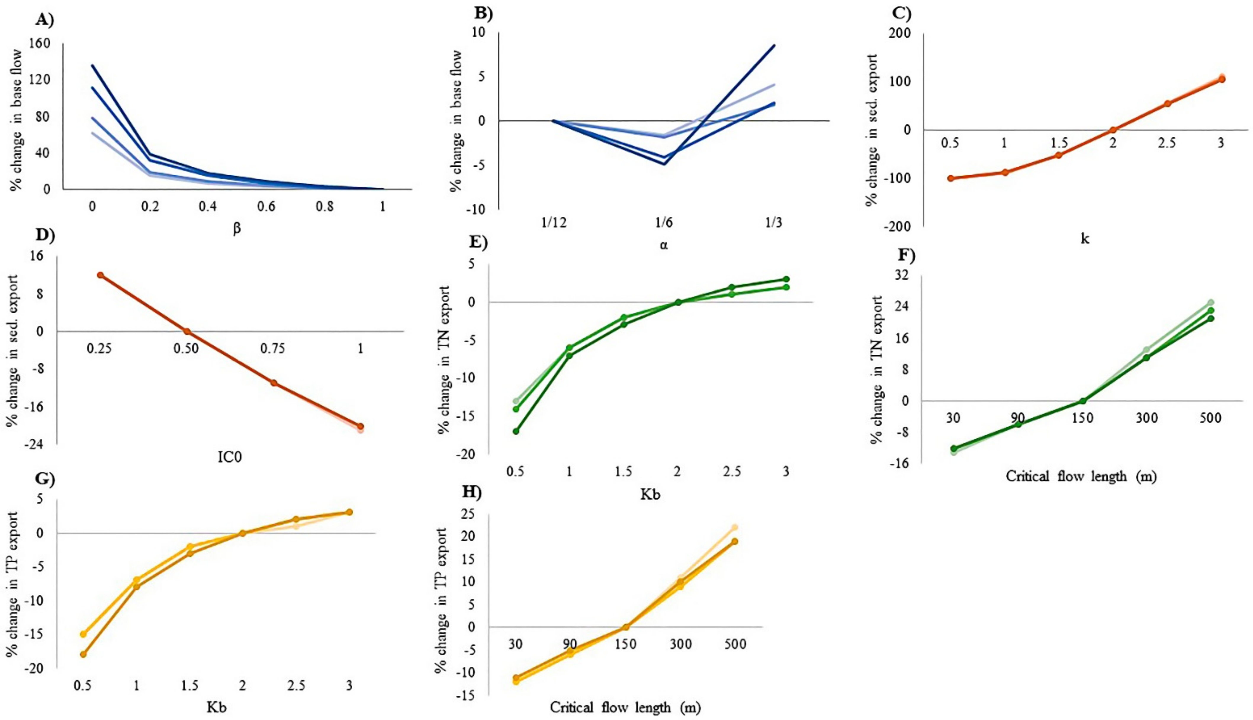
The sensitivity analysis of the SWY model parameters indicated that β is the most sensitive and has the greatest influence on BF variation (Figure 3). Increased β values decreased BF in all sub-basins, primarily, in the range of values that varies between 0 ≤ β < 0.4. Compared to the default values, reduction in the value of β to 0.2 increases BF 26% on average, with the greatest variation (39%) in sub-basin SF-IV. For α, however, the trends varied. BF decreased by an average of 3% to α = 1/6 and increased by an average of 5% to α = 1/3, chiefly in sub-basin SF-IV, where the average increase was approximately 10%.
Sediment export in the SDR model showed greater sensitivity for parameter kb, whose increase is associated with greater sediment export to all sub-basins (Figure 3). For kb = 0.5, the exported sediment value is on average 100% lower than the default value, and for kb = 3, the value is on average 107% higher. In absolute values (t yr−1), the highest sensitivity occurs between 0.5 ≤ kb ≤ 1, where the sediment exported for k = 1 is 34 times greater. Values between 1.5 ≤ kb ≤ 2.5 tend to vary sediment export by approximately −50% and +50%, respectively. Changes in IC0 values showed lower sensitivity and opposite behavior compared to kb variations. The increase in IC0 values is related to a lower sediment export. On average, an increase of 0.25 in IC0 values tends to decrease the value of exported sediment by 11%. Compared to the default value, the value of IC0 = 1 provided an increase of 20% of the sediment exported to all sub-basins, while the value of IC0 = 0.25 decreased by 12%.
The sensitivity of the parameters k and critical flow length showed the same behavior for TP and TN (Figure 3). In general, nutrient exports were more sensitive to changes in critical flow length values. This study considered the value of 150 m as the default for this parameter, decreasing this value to 30 m provided a reduction of approximately 12% in the value of exported nutrients, while the value of 500 m increased by almost 25%. The parameter k was more sensitive between 0.5 ≤ k ≤ 1 and its effect is more expressive in the decrease of nutrient export than in the increase. Relative to the default value (k = 2), decreasing to k = 0.5 decreased nutrient export by 15%, while changing to k = 3 showed a slight increase of almost 3%.
3.2. Calibration and Validation of WES Temporal Variability
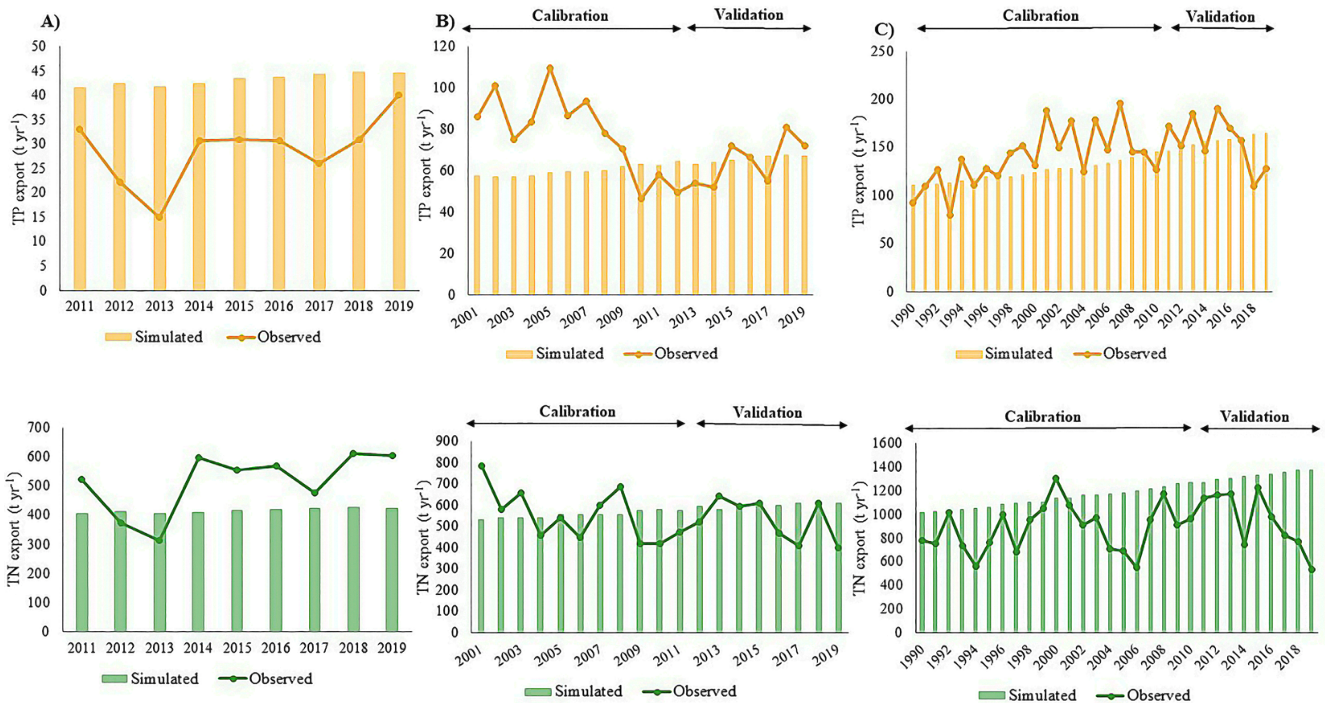
The SWY, SDR, and NDR models perform differently in the spatial and temporal scales. Figure 4, Figure 5 and Figure 6 show the simulated and observed WES values over time and the models’ adjusted parameter values. Table 2 presents performance indicators. The best calibration and validation performance was observed for the SWY model. A visual comparison of the simulated and observed annual streamflow indicates a good fit for all sub-basins (Figure 4). Although the best performance involved values close to the long-term annual averages, the model was able to represent streamflow variation over time. R2 indicated an acceptable performance for the calibration period, but NSE was unsatisfactory for all sub-basins. PBIAS indicated that the SWY model underestimated annual streamflow in sub-basins SF-I and SF-IV and overestimated it in sub-basins SF-II and SF-III, with very good and good performance, respectively. For the validation period, R2 values indicated satisfactory to acceptable performances. NSE values indicated satisfactory performance and PBIAS values presented different values for each sub-basin, with unsatisfactory performance observed in sub-basin SF-II and very good performance in sub-basin SF-III.
The SDR model effectively represented years with values close to the long-term average, but did not perform well in representing the annual variability of exported sediment (Figure 5). The results indicated large discrepancies for specific years, but those between the observed and simulated values were not systemic. NSE and R2 values for the calibration and validation period reflected the SDR model’s limited capacity to represent the annual variability of exported sediment, indicating inconsistent performance (Table 2). PBIAS values showed that the SDR model overestimated the sediment load exported annually in the calibration period, with very good performance in sub-basins WQ-I and WQ-II and good performance for sub-basin WQ-III. PBIAS found varying trends in the sub-basins for the validation period, underestimating the sediment load exported in sub-basin WQ-II and overestimating it in sub-basin WQ-III, with satisfactory and good performance, respectively (Table 2).
Nutrients simulated by the NDR model present higher performance for values close to the long-term mean of the observed data. However, unlike the SWY and SDR models, the NDR model is unable to represent the annual variability of nutrient loads (Figure 6). For TP and TN, values tend to remain close to the average, showing a slight variation over time. Concerning the NDR model’s performance, the adjustment of the calibration parameters showed high variability among sub-basins. With regard to the values of the annual TP loads for the calibration and validation period, the R2 and NSE indicators indicated unsatisfactory performance for all sub-basins (Table 2). Although R2 was increased for sub-basin WQ-II (R2 = 0.6) in the calibration period, the analysis found an inversely proportional relationship between the simulated and observed data, which indicates the model’s inconsistent performance. PBIAS, however, indicated satisfactory performance in the calibration period for sub-basin WQ-III and very good performance for the validation period in sub-basins WQ-II and WQ-III (Table 2). The performance indicators obtained for modeled TN annual loads showed the same trend as for modeled TP annual loads. The PBIAS indicator indicated very good and satisfactory performances only in sub-basin WQ-II for the calibration and validation period, respectively (Table 2).
3.3. WES Spatial Performance Analysis
SWY model results demonstrated a reasonable fit with the observed data (Table 3). R2 indicated acceptable performance, and the PBIAS and NSE indicators demonstrated a very good and unsatisfactory performance, respectively. For the SDR, NDR-TN, and NDR-TP models, PBIAS indicated a performance ranging from satisfactory to very good, while the other indicators showed unsatisfactory performance.
The study’s results indicate that, in general, the models were able to simulate the long-term mean values observed in the sub-basins (Table 4). The largest discrepancy occurred in sub-basin WQ-I for the NDR-TP model, and the smallest discrepancy was observed in sub-basin SF-I for the SWY model.
4. Discussion
4.1. WES Sensitivity Analysis
Unlike other studies that analyzed the sensitivity of calibration parameters and input data [27,60,61], this study examined just the calibration parameters’ sensitivity, choosing not to analyze the sensitivity of the input data because the vast bulk came from monitoring stations, which tend to have higher quality than other databases. When feasible, empirical values were also used for some input parameters, such as soil erodibility and crop and nutrient export coefficients, which best represent the characteristics of the studied area.
With regard to the SWY model, the study indicated the β parameter as the most sensitive, having a significant effect on flow routing and, consequently, on BF values. Hamel et al. [28] also found greater sensitivity for β, with BF varying by nearly 50% in some sub-basins. For α = 1/12 and α = 1/6, the decreasing BF was similar to Hamel et al. [28], but for alpha = 1/3, there was a BF increase (Figure 3), associated with the determination of AETi,m, which is conditioned by PET or water availability, according to Equation (4). The parameters α and β are associated with the fraction of the annual recharge of pixels upstream (upslope) available for evapotranspiration of a pixel downstream (downslope) [16]. The configuration of alpha = 1/3 and beta = 1 (default value) renders the potential available water (Lsum.avail,i), very high, requiring the algorithm to use PETi,m to calculate AETi,m (Equation (4)).
The sensitivity of the SDR model parameters k and IC0 followed that of Hamel et al. [25], as anticipated in light of the model’s configuration [16]. Although both parameters characterize the relationship between the connectivity index and sediment delivery rate, the sensitivity of k was greater than that of IC0, with higher values associated with a higher sediment delivery rate, as predicted by Vigiak et al. [53], suggesting that k variations are more effective for data calibration and validation. The result of the sensitivity analysis of the IC0 parameter appears more sensitive than that in Hamel et al. [25], although it showed the same linear decrease in exported sediment.
For the NDR model, the sensitivity of the parameter k occurred as anticipated, given the relationship between nutrient export and k is generally exponential when k is less than nine and linear when it is greater [62]. As noted in other studies [27,62], the results of this research showed that the parameter k is most sensitive between the values of 0 ≤ k ≤ 1, in which the projected curve presents sigmoidal behavior, that is, an expressive increase at the onset and a tendency to stabilize as k values increase. In this study, the effect of k in all sub-basins was similar (Figure 3) as a result of basin’s hydrogeological similarity. However, as demonstrated by Redhead et al. [27], the response in k variations is specific to each location, and thus may differ from the results herein. Variations in critical flow length values indicate a directly proportional linear relationship with the exported nutrient load. This was also expected, since it is assumed that the greater the distance for a land-use fragment to reach its maximum retention capacity, the greater the probability of the nutrient load reaching the watershed [16].
4.2. InVEST WES Model Performance
The study’s sensitivity analysis increases our understanding of the effect of calibration parameters on the modeled results and how to optimize their representation of the observed data, which its performance analysis indicates the InVEST WES models are reasonably effective in simulating, albeit with high variability according to the model and analysis scale. Using the SWAT model and the Generalized Watershed Loading Function, Santos et al. [63] modeled the streamflow and sediment and nutrient loads in the upper part of the basin with results analogous to those herein, with both indicating improved performance in simulating streamflow.
With regard to the InVEST WES models’ calibration and temporal validation, the best performance was observed for the SWY model. Despite some indicators of unsatisfactory performance, particularly in the calibration period for NSE, the results show that the model was able to represent the temporal variability of the average annual streamflow in the sub-basins for the calibration and validation period (Figure 4 and Table 2). The effective performance of the SWY model may be associated with its high sensitivity to variations in precipitation, as noted in the literature [29,61]. Likewise, the inferior performance of the NDR and SDR models may be related to their lower sensitivity [27,64,65]. Insensitivity to precipitation in UK watersheds [27] is inherent in the NDR model’s configuration (Equation (16)), where its sole effect is to modify the nutrient load’s impact on surface runoff, based on an index that relates pixel precipitation to the basin’s average rainfall. That is, the effect of precipitation is more closely associated with its configuration than with its intensity. In the SDR model, as opposed to the NDR, precipitation has a greater expressive influence on sediment export (Figure 5) because rainfall erosivity is key to triggering erosion (Equation (9)). Some studies have indicated high sensitivity to erosivity in the SDR model [25,66]. Although this study used annual rainfall and land-use data as model inputs, temporal variability was not well captured by the SDR and NDR models.
The spatial performance of InVEST’s WES models is often evaluated using long-term average values. Due to the dearth of monitoring stations, this study included all values in the historical series sampled in the basin to calculate the statistical indicators and evaluate the spatial performance of the models. Although not detailed herein, it should be noted that an initial analysis was conducted, using WES values not normalized by the drainage area, which deemed the performance of all models good. However, as the study’s objective was to examine the models’ capacity to forecast WES behavior in the basin, taking into account the variability of land use patterns, specific WES values were used, and the models’ spatial performances were significantly reduced (Table 3).
When compared with observed long-term mean values, the results were similar to those in the literature [13,24,25,27,28], indicating that the InVEST WES models yield good results in terms of relative magnitude. The SWY model performed best, with simulated long-term average flow deviations of less than 10% from observed values. These results confirm the findings of other studies that have shown reasonable performance for the SWY model [13,28,29]. The long-term average loads of exported sediments simulated by the SDR model also showed limited discrepancies with observed values, corroborating studies that have featured its potential to simulate sediment dynamics [24,25,66]. The greatest deviations in NDR model simulations were found in sub-basins WQ-I and WQ-III, which overestimated TN and TP exports by 50% and 32%, respectively. Redhead et al. [27] obtained similar results in UK watersheds, with the vast majority showing deviations from observed values for TN and TP of 65% and 44%, respectively.
In calibrating the models, it could be seen that that the values assigned to the calibration parameters generally reflected the hydrogeological characteristics of the basin, which is located in a flat region, in which some 80% of the relief is composed of smoothly undulating hills with low drainage density [43], with a slope around 8%. The basin’s soils are primarily sandy and deep (~75%), as is characteristic of Brazil’s Cerrado biome. Thus, the basin has a low potential to generate surface runoff and, consequently, to transport nutrients and of sediments to watercourses. The values assigned to the calibration parameters reflected these characteristics.
In the SWY model, the values β = 0.2 and α = 1/12 presented the best relationship with observed values and increased the BF share of water yield, conditions that occur in regions with flat, smooth topography. Their determination is consistent for the basin as it is an important recharge area for the Guarani Aquifer, one of the largest underground freshwater reservoirs in the world [41,42]. The values assigned to the SDR model parameters (k = 0.8 and IC0 = 0.45) also reflect the basin’s environmental characteristics, characterizing environments with low potential for sediment transport, although their soils are highly susceptible to erosion [57,67]. The NDR model-TP was the only one in which the default value of the calibration parameter was maintained (k = 2), although the transport of nutrients was reduced through the critical flow length parameter.
4.3. InVEST WES Model Potentials and Limitations
InVEST’s WES models present simple approaches and demand few input data compared to other physical-based hydrological models, such as SWAT. These characteristics facilitate decision making in non-instrumented basins or regions where data is scarce, as demonstrated by Benra et al. [13] and corroborated by this study. InVEST’s WES models enable spatial understanding since they are distributed at pixel scale, and the WES value in each pixel varies depending on its location, considering such key factors as land use, vegetation, relief, and soil types, which remain a major challenge for ecohydrological models [68,69]. Such characteristics make these models important tools for environmental planning, enabling an analysis of the effects of diverse future scenarios, such as climate and land-use changes, the primary drivers of WES degradation [4,5]. While WES model performance differs for each model and temporal and spatial scale, in general, the study results indicate the models’ capacity to represent long-term average values, and, in the case of the SWY model, to simulate annual average values, enabling a representation of the variability of extreme annual values (see 1983 in Figure 4).
Like any other model, InVEST’s WES models have advantages and limitations. Accordingly, further research to enhance them and increase their transparency is in order. As noted in the InVEST manual, the models use simple equations and limited parameters to estimate water ecosystems services [16]. An analysis of the results of this study confirm the limitations noted in the InVEST user manual and in other studies [16,25,27]. The principal limitation of the SWY model is its inability to accurately represent water flow, that is, surface runoff and base flow. The discrepancies arise from its simulation of surface runoff, based on an adaptation of the SCS curve number method, which disregards topographical effects, and of base flow, whose simplified routing equations can generate inconsistent results in terms of absolute numbers [70]. It should also be noted the model fails to simulate the annual variability of water yield in the watershed. Although it enables evaluation of the monthly surface runoff, this limits its use to contexts that demand data on a more refined time scale, as in the simulation of reference streamflow to calculate water availability [71].
The effect of simplification is even more significant in the SDR and NDR models, which are even more sensitive to input data. Uncertainties related to input parameters, such as R and K from RUSLE, and export and nutrient retention coefficients can have considerable impact on the models’ simulations [16,25]. In many regions, there is no information available on these empirically determined parameters, necessitating the use of data from other locations, which may have quite different climatic and hydrogeological characteristics.
Other limitations associated with the generalization of complex physical processes relate to nutrient and sediment dynamics. In the SDR model, sediment yield is solely determined by RUSLE, disregarding such sources as the gully, stream bank, and mass erosion, which are useful in comparing simulations with observations [25]. The determination of TN and TP loads in the NDR model disregards the cycle of each nutrient, quantifying both loads in the same way through the relationship between land-use and export coefficients, a considerable abstraction given that their environmental dynamics are quite different [72]. Neither the SDR nor NDR model take into account the dynamics of nutrients and sediments in watercourses, assuming that the entire load that enters the watercourses is exported to the watershed. The NDR model does not take into account point loads, which can adversely impact urbanized basins, especially in areas where basic sanitation is deficient. In the basin, for example, where urban areas represent only 4% of the area, points contribute, on average, up to 60% of the total loads.
4.4. Potential, Uncertainties, and Limitations
Unlike most studies that analyzed the spatial performance of InVEST’s WES models, considering long-term average values [13,24,25,26,27,28], this study analyzes their performance, considering WES spatial and temporal variability. Of the studies reviewed, only Lu et al. [29] analyzed the temporal performance of the SWY model using Pearson’s correlation, albeit using a brief historical series of observed flow data. This study uses historic series of land-use and meteorological data measured at monitoring stations to simulate the temporal variability of WES, considering climate and land use, which exert significant influence on WES dynamics in hydrographic basins.
The principal uncertainties pertaining to the study’s calibration method pertain to the use of historical series of observed data. The daily and monthly streamflow data, for example, had numerous flaws, and several stations lacked data for the complete series (1981–2019). With regard to TN, TP, and TSS water quality data, it should be noted that CETESB samples are only taken every two months. In addition, many CETESB monitoring stations do not perform streamflow measurements at the points where water quality samples are taken, which makes determining nutrient and sediment loads needed for comparison with model results problematic. An attempt was made to circumvent flow data deficiencies using hydrological regionalization, and the effects of limited annual sampling and, consequently, the seasonality of the water quality data, were reduced by removing outliers (see Section 2.5), since bi-monthly measurements do not represent the annual TN, TP, and TSS averages. Thus, despite strenuous efforts to calibrate and validate the WES models, uncertainties and limitations remain.
In addition to such challenges with observed data, there are uncertainties related to the empirical parameters used in the models. The study sought to use regional data for all parameters, since they best represent the environmental characteristics of the basin studied (see Supplementary Material). However, for some parameters, such as CN and nutrient retention efficiency coefficients, for example, it was not feasible to use empirical values, which can contribute to uncertainty in model results. For the NDR model, uncertainties include quantification of TN and TP point loads, estimated from on the per capita load of domestic sewage, using export coefficients, population data, and nutrient removal coefficients, and the values are uncertain due to the scarcity of data on basic sanitation in the basin’s municipalities.
5. Conclusions
This study investigated the performance of InVEST 3.9.0 WES models, analyzing their ability to represent the spatial and temporal variability of observed values. The results show a high variability in their performances, according to the type of water ecosystem services simulated and scales of analysis. The best performance was observed for the SWY model, which effectively represented the spatial and temporal variability of the average annual streamflow in the analyzed sub-basins. The SDR and NDR models were unable to represent the temporal variability of the exported loads of sediments and nutrients. The inferior performance of these models may be associated with lower sensitivity to precipitation variability. The NDR model, in particular, appears insensitive to annual variations in precipitation, which impact the annual load of nutrients exported in the basin.
The spatial performance considering specific WES values was low for most statistical indicators. In general, with the exception of some sub-basins, all models showed good performance in simulating long-term mean values, which corroborates the results of other studies.
Properly calibrating models’ parameters is essential to enhancing their performance, and the values the study assigned to them reflected the basin’s hydrogeological characteristics. Uncertainties regarding the methodology used for calibration and validation relate to the quality of the historical series of observed data of daily and monthly streamflow and inadequate water quality sampling data, as well as the failure to measure streamflow data. While the study attempted to circumvent such obstacles, uncertainties remain, and the results should be interpreted with circumspection. Furthermore, some findings may be solely empirical, as the study area lacks broad hydrogeological variability.
Despite the uncertainties and empirical nature of this study, its results and discussions should aid researchers and other users of InVEST models to inform and make decisions and formulate policies. To minimize uncertainties and enhance results, the use of the complete historical series of streamflow and, particularly of water quality parameters is recommended to better reflect the basin’s hydrological characteristics and correspond to simulated data. In as much as the performance of the models may vary according to the hydrogeological nature of the region in which they are being applied, further research in varied basins in diverse regions should be conducted to complement the findings detailed herein.
Supplementary Materials
The following supporting information can be downloaded at: https://www.mdpi.com/article/10.3390/w14101559/s1, Equation (S1): Camargo method for evapotranspiration; Equation (S2): rainfall erosivity; Equation (S3): LS factor; Equation (S4): nutrient loads; Equation (S5): point loads; Table S1: biophysical table for the SWY model; Table S2 biophysical tables for SDR and NDR models [5,26,32,34,52,54,73,74,75,76,77,78,79,80,81,82,83,84,85,86,87].
Author Contributions
Conceptualization, P.d.S.A.; methodology, P.d.S.A. and M.A.G.A.B.; investigation, P.d.S.A.; writing—original draft preparation, P.d.S.A.; and writing—review and editing P.d.S.A., M.A.G.A.B. and F.F.M.; supervision, F.F.M. All authors have read and agreed to the published version of the manuscript.
Funding
This research is supported by the National Council of Scientific and Technological Development (CNPq grant 140518/2019-3).
Institutional Review Board Statement
Not applicable.
Informed Consent Statement
Not applicable.
Data Availability Statement
The hydrological data are publicity available at <https://www.snirh.gov.br/; http://www.daee.sp.gov.br/site/>, meteorological data at < https://www.snirh.gov.br/>, water quality at <https://sistemainfoaguas.cetesb.sp.gov.br/>, land-use data at < http://mapbiomas.org/>, and DEM data at < https://vertex.daac.asf.alaska.edu>. Data were accessed between May and August 2021.
Conflicts of Interest
The authors declare no conflict of interest.
References
- Grizzetti, B.; Lanzanova, D.; Liquete, C.; Reynaud, A.; Cardoso, A.C. Assessing Water Ecosystem Services for Water Resource Management. Environ. Sci. Policy 2016, 61, 194–203. [Google Scholar] [CrossRef]
- Brauman, K.A.; Daily, G.C.; Duarte, T.K.E.; Mooney, H.A. The Nature and Value of Ecosystem Services: An Overview High-Lighting Hydrologic Services. Annu. Rev. Environ. Resour. 2007, 32, 67–98. [Google Scholar] [CrossRef]
- Palomo, I.; Bagstad, J.K.; Nedkov, S.; Klug, H.; Adamescu, M.; Cazacu, C. Tools for Mapping Ecosystem Services. In Mapping Ecosystem Services; Pensoft Publishers: Sofia, Bulgaria, 2017; p. 70. [Google Scholar]
- Bucak, T.; Trolle, D.; Tavşanoğlu, Ü.N.; Çakıroğlu, A.İ.; Özen, A.; Jeppesen, E.; Beklioğlu, M. Modeling the Effects of Climatic and Land Use Changes on Phytoplankton and Water Quality of the Largest Turkish Freshwater Lake: Lake Beyşehir. Sci. Total Environ. 2018, 621, 802–816. [Google Scholar] [CrossRef] [PubMed]
- Bai, Y.; Ochuodho, T.O.; Yang, J. Impact of Land Use and Climate Change on Water-Related Ecosystem Services in Kentucky, USA. Ecol. Indic. 2019, 102, 51–64. [Google Scholar] [CrossRef]
- Ferreira, P.; van Soesbergen, A.; Mulligan, M.; Freitas, M.; Vale, M.M. Can Forests Buffer Negative Impacts of Land-Use and Climate Changes on Water Ecosystem Services? The Case of a Brazilian Megalopolis. Sci. Total Environ. 2019, 685, 248–258. [Google Scholar] [CrossRef]
- Kadaverugu, A.; Rao, C.N.; Viswanadh, G.K. Quantification of Flood Mitigation Services by Urban Green Spaces using InVEST Model: A Case Study of Hyderabad City, India. Modeling Earth Syst. Environ. 2021, 7, 589–602. [Google Scholar] [CrossRef]
- Feld, C.K.; Birk, S.; Bradley, D.C.; Hering, D.; Kail, J.; Marzin, A.; Pont, D. From Natural to Degraded Rivers and Back Again: A 1248 Test of Restoration Ecology Theory and Practice. Adv. Ecol. Res. 2011, 44, 119–209. [Google Scholar] [CrossRef]
- Li, T.; Lü, Y.; Fu, B.; Hu, W.; Comber, A.J. Bundling Ecosystem Services for Detecting Their Interactions Driven by Large-Scale Vegetation Restoration: Enhanced Services While Depressed Synergies. Ecol. Indic. 2019, 99, 332–342. [Google Scholar] [CrossRef] [Green Version]
- Lara, A.; Jones, J.; Little, C.; Vergara, N. Streamflow Response to Native Forest Restoration in Former Eucalyptus Plantations in South Central Chile. Hydrol. Processes 2021, 35, e14270. [Google Scholar] [CrossRef]
- Souza, A.R.; Dupas, F.A.; da Silva, I.A. Spatial Targeting Approach for a Payment for Ecosystem Services Scheme in a Peri-Urban Wellhead Area in Southeastern Brazil. Environ. Chall. 2021, 5, 100206. [Google Scholar] [CrossRef]
- Hrachowitz, M.; Savenije, H.H.G.; Blöschl, G.; McDonnell, J.J.; Sivapalan, M.; Pomeroy, J.W.; Cudennec, C. A Decade of Predictions in Ungauged Basins (PUB)—A Review. Hydrol. Sci. J. 2013, 58, 1198–1255. [Google Scholar] [CrossRef]
- Benra, F.; De Frutos, A.; Gaglio, M.; Álvarez-Garretón, C.; Felipe-Lucia, M.; Bonn, A. Mapping Water Ecosystem Services: Evaluating InVEST Model Predictions in Data Scarce Regions. Environ. Model. Softw. 2021, 138, 104982. [Google Scholar] [CrossRef]
- Villa, F.; Ceroni, M.; Bagstad, K.; Johnson, G.; Krivov, S. ARIES (Artificial Intelligence for Ecosystem Services): A New Tool for Ecosystem Services Assessment, Planning, and Valuation. In Proceedings of the 11th Annual BIOECON Conference on Economic Instruments to Enhance the Conservation and Sustainable Use of Biodiversity, Venice, Italy, 21–22 September 2009; pp. 21–22. [Google Scholar]
- Boumans, R.; Roman, J.; Altman, I.; Kaufman, L. The Multiscale Integrated Model of Ecosystem Services (MIMES): Simulating the Interactions of Coupled Human and Natural Systems. Ecosyst. Serv. 2015, 12, 30–41. [Google Scholar] [CrossRef]
- Sharp, R.; Douglass, J.; Wolny, S.; Arkema, K.; Bernhardt, J.; Bierbower, W.; Chaumont, N.; Denu, D.; Fisher, D.; Glowinski, K.; et al. InVEST 3.9.0. User’s Guide. The Natural Capital Project; Stanford University: Stanford, CA, USA, 2020. [Google Scholar]
- Arnold, J.G.; Moriasi, D.N.; Gassman, P.W.; Abbaspour, K.C.; White, M.J.; Srinivasan, R.; Kannan, N. SWAT: Model Use, Calibration, and Validation. Trans. ASABE 2012, 55, 1491–1508. [Google Scholar] [CrossRef]
- Liang, X.; Lettenmaier, D.P.; Wood, E.F.; Burges, S.J. A Simple Hydrologically Based Model of Land Surface Water and Energy Fluxes for General Circulation Models. J. Geophys. Res. Atmos. 1994, 99, 14415–14428. [Google Scholar] [CrossRef]
- Tague, C.L.; Band, L.E. Regional Hydro-Ecologic Simulation System—An Object-Oriented Approach to Spatially Distributed Modeling of Carbon, Water, and Nutrient Cycling. Earth Interact. 2004, 8, 1–42. [Google Scholar] [CrossRef]
- Keeler, B.L.; Polasky, S.; Brauman, K.A.; Johnson, K.A.; Finlay, J.C.; O’Neill, A.; Dalzell, B. Linking Water Quality and Well-Being for Improved Assessment and Valuation of Ecosystem Services. Proc. Natl. Acad. Sci. USA 2012, 109, 18619–18624. [Google Scholar] [CrossRef] [Green Version]
- Vigerstol, K.L.; Aukema, J.E. A Comparison of Tools for Modeling Freshwater Ecosystem Services. J. Environ. Manag. 2011, 92, 2403–2409. [Google Scholar] [CrossRef]
- Jorda-Capdevila, D.; Gampe, D.; García, V.H.; Ludwig, R.; Sabater, S.; Vergoñós, L.; Acuña, V. Impact and Mitigation of Global Change on Freshwater-Related Ecosystem Services in Southern Europe. Sci. Total Environ. 2019, 651, 895–908. [Google Scholar] [CrossRef]
- Yang, S.; Zhao, W.; Liu, Y.; Wang, S.; Wang, J.; Zhai, R. Influence of Land Use Change on the Ecosystem Service Trade-Offs in the Ecological Restoration Area: Dynamics and Scenarios in the Yanhe Watershed, China. Sci. Total Environ. 2018, 644, 556–566. [Google Scholar] [CrossRef] [PubMed]
- Terrado, M.; Acuña, V.; Ennaanay, D.; Tallis, H.; Sabater, S. Impact of Climate Extremes on Hydrological Ecosystem Services in a Heavily Humanized Mediterranean Basin. Ecol. Indic. 2014, 37, 199–209. [Google Scholar] [CrossRef]
- Hamel, P.; Chaplin-Kramer, R.; Sim, S.; Mueller, C. A New Approach to Modeling the Sediment Retention Service (InVEST 3.0): Case Study of the Cape Fear Catchment, North Carolina, USA. Sci. Total Environ. 2015, 524, 166–177. [Google Scholar] [CrossRef]
- Redhead, J.W.; Stratford, C.; Sharps, K.; Jones, L.; Ziv, G.; Clarke, D.; Bullock, J.M. Empirical Validation of the InVEST Wateryield Ecosystem Service Model at a National Scale. Sci. Total Environ. 2016, 569, 1418–1426. [Google Scholar] [CrossRef] [PubMed] [Green Version]
- Redhead, J.W.; May, L.; Oliver, T.H.; Hamel, P.; Sharp, R.; Bullock, J.M. National Scale Evaluation of the InVEST Nutrient Retention Model in the United Kingdom. Sci. Total Environ. 2018, 610, 666–677. [Google Scholar] [CrossRef] [PubMed]
- Hamel, P.; Valencia, J.; Schmitt, R.; Shrestha, M.; Piman, T.; Sharp, R.P.; Guswa, A.J. Modeling Seasonal Water Yield for Landscape Management: Applications in Peru and Myanmar. J. Environ. Manag. 2020, 270, 110792. [Google Scholar] [CrossRef] [PubMed]
- Lu, H.; Yan, Y.; Zhu, J.; Jin, T.; Liu, G.; Wu, G.; Stringer, L.C.; Dallimer, M. Spatiotemporal Water Yield Variations and Influencing Factors in the Lhasa River Basin, Tibetan Plateau. Water 2020, 12, 1498. [Google Scholar] [CrossRef]
- Hackbart, V.C.; De Lima, G.T.; Dos Santos, R.F. Theory and Practice of Water Ecosystem Services Valuation: Where Are We Going? Ecosyst. Serv. 2017, 23, 218–227. [Google Scholar] [CrossRef]
- Willcock, S.; Hooftman, D.; Sitas, N.; O’Farrell, P.; Hudson, M.D.; Reyers, B.; Bullock, J.M. Do Ecosystem Service Maps and Models Meet Stakeholders’ Needs? A Preliminary Survey across Sub-Saharan Africa. Ecosyst. Serv. 2016, 18, 110–117. [Google Scholar] [CrossRef] [Green Version]
- Manhães, A.P.; Mazzochini, G.G.; Oliveira-Filho, A.T.; Ganade, G.; Carvalho, A.R. Spatial Associations of Ecosystem Services and Biodiversity as a Baseline for Systematic Conservation Planning. Divers. Distrib. 2016, 22, 932–943. [Google Scholar] [CrossRef]
- Saad, S.I.; Mota da Silva, J.; Silva, M.L.N.; Guimarães, J.L.B.; Sousa, W.C., Jr.; Figueiredo, R.D.O.; Rocha, H.R.D. Analyzing Ecological Restoration Strategies for Water and Soil Conservation. PLoS ONE 2018, 13, e0192325. [Google Scholar] [CrossRef] [Green Version]
- Resende, F.M.; Cimon-Morin, J.; Poulin, M.; Meyer, L.; Loyola, R. Consequences of Delaying Actions for Safeguarding Ecosystem Services in the Brazilian Cerrado. Biol. Conserv. 2019, 234, 90–99. [Google Scholar] [CrossRef]
- Rosário, V.A.; Guimarães, J.C.; Viani, R.A. How Changes in Legally Demanded Forest Restoration Impact Ecosystem Services: A Case Study in the Atlantic Forest, Brazil. Trop. Conserv. Sci. 2019, 12, 1940082919882885. [Google Scholar] [CrossRef]
- Gomes, L.C.; Bianchi, F.J.; Cardoso, I.M.; Fernandes Filho, E.I.; Schulte, R.P. Land Use Change Drives the Spatio-Temporal Variation of Ecosystem Services and Their Interactions along an Altitudinal Gradient in Brazil. Landsc. Ecol. 2020, 35, 1571–1586. [Google Scholar] [CrossRef]
- Hamel, P.; Bremer, L.L.; Ponette-González, A.G.; Acosta, E.; Fisher, J.R.; Steele, B.; Brauman, K.A. The Value of Hydrologic Information for Watershed Management Programs: The Case of Camboriú, Brazil. Sci. Total Environ. 2020, 705, 135871. [Google Scholar] [CrossRef] [PubMed]
- Saad, S.I.; da Silva, J.M.; Ponette-González, A.G.; Silva ML, N.; da Rocha, H.R. Modeling the On-Site and Off-Site Benefits of Atlantic Forest Conservation in a Brazilian Watershed. Ecosyst. Serv. 2021, 48, 101260. [Google Scholar] [CrossRef]
- CBH-TJ. Tietê Jacaré River Hydrographic Basin Committee. UGRHI 13 River Basin Plan. Technical Document, São Paulo, Brazil. 2016. Available online: https://sigrh.sp.gov.br/ (accessed on 22 July 2021).
- Peel, M.C.; Finlayson, B.L.; McMahon, T.A. Updated World Map of the Köppen-Geiger Climate Classification. Hydrol. Earth Syst. Sci. 2007, 11, 1633–1644. [Google Scholar] [CrossRef] [Green Version]
- Costa, C.W.; Lorandi, R.; Lollo, J.A.; Santos, V.S. Potential for Aquifer Contamination of Anthropogenic Activity in the Recharge Area of the Guarani Aquifer System, Southeast of Brazil. Groundw. Sustain. Dev. 2019, 8, 10–23. [Google Scholar] [CrossRef]
- Lucas, M.; Wendland, E. Recharge Estimates for Various Land Uses in the Guarani Aquifer System Outcrop Area. Hydrol. Sci. J. 2016, 61, 1253–1262. [Google Scholar] [CrossRef]
- Rossi, M. Mapa Pedológico do Estado de São Paulo: Revisado e Ampliado; Instituto Florestal: São Paulo, Brasil, 2017; Volume 1, p. 118. [Google Scholar]
- Trevisan, D.P.; Ruggiero, M.H.; Bispo PD, C.; Almeida, D.; Imani, M.; Balzter, H.; Moschini, L.E. Evaluation of Environmental Naturalness: A Case Study in the Tietê-Jacaré Hydrographic Basin, São Paulo, Brazil. Sustainability 2021, 13, 3021. [Google Scholar] [CrossRef]
- MapBiomas. Brazil Land Use Data Series. Collection 5, Brazil. 2021. Available online: https://mapbiomas.org/colecoes-mapbiomas-1?cama_set_language=pt-BR (accessed on 13 July 2021).
- ASF. Alaska Satellite Facility. ALOS-PALSAR Images. 2021. Available online: https://vertex.daac.asf.alaska.edu (accessed on 5 May 2021).
- ANA. National Water and Sanitation Agency. Hydrological Information System (HidroWeb), Brasilia, Brazil. 2021. Available online: https://www.snirh.gov.br/hidroweb/apresentacao (accessed on 15 August 2021).
- DAEE. Department of Water and Electric Energy. Hydrological database, Sao Paulo, Brazil. 2021. Available online: http://www.daee.sp.gov.br/site/ (accessed on 22 August 2021).
- CETESB. São Paulo State Environmental Company. Information System InfoÁGUAS, Sao Paulo, Brazil. 2021. Available online: https://sistemainfoaguas.cetesb.sp.gov.br/ (accessed on 20 August 2021).
- NRCS. Urban Hydrology for Small Watersheds-Technical Release 55; US Department of Agriculture Natural Resources Conservation: Washington, DC, USA, 1986. [Google Scholar]
- Borselli, L.; Cassi, P.; Torri, D. Prolegomena to Sediment and Flow Connectivity in the Landscape: A GIS and Field Numerical Assessment. Catena 2008, 75, 268–277. [Google Scholar] [CrossRef]
- Mannigel, A.R.; de Passos, M.; Moreti, D.; da Rosa Medeiros, L. Fator Erodibilidade e Tolerância de Perda dos Solos do Estado de São Paulo. Acta Scientiarum. Agron. 2002, 24, 1335–1340. [Google Scholar] [CrossRef]
- Vigiak, O.; Borselli, L.; Newham, L.T.H.; McInnes, J.; Roberts, A.M. Comparison of Conceptual Landscape Metrics to Define Hillslope-Scale Sediment Delivery Ratio. Geomorphology 2012, 138, 74–88. [Google Scholar] [CrossRef]
- SMA. Secretariat for the Environment of the State of São Paulo. Billings Reservoir Watershed Development and Environmental Protection Plan, Sao Paulo, Brazil. 2010. Available online: https://www.infraestruturameioambiente.sp.gov.br/cpla/2013/03/aprm-billings/ (accessed on 23 August 2021).
- IBGE. Brazilian Institute of Geography and Statistics. Metadados. 2021. Available online: https://metadados.geo.ibge.gov.br/ (accessed on 27 July 2021).
- Anjinho, P.S.; Barbosa MA, G.A.; Neves, G.L.; Dos Santos, A.R.; Mauad, F.F. Integrated Empirical Models to Assess Nutrient Concentration in Water Resources: Case Study of a Small Basin in Southeastern Brazil. Environ. Sci. Pollut. Res. 2021, 28, 23349–23367. [Google Scholar] [CrossRef] [PubMed]
- Anjinho, P.S. Distributed Modeling of Point and Diffuse Pollution of the Water Systems of the Lobo Stream Watershed, Itirapina-SP. Master’s Thesis, University of Sao Paulo, São Carlos, São Paulo, Brazil, 2019. Available online: https://teses.usp.br/teses/disponiveis/18/18139/tde-13052019-164214/pt-br.php (accessed on 27 July 2021).
- Nash, J.E.; Sutcliffe, J.V. River Flow Forecasting through Conceptual Models Part I—A Discussion of Principles. J. Hydrol. 1970, 10, 282–290. [Google Scholar] [CrossRef]
- Rauf, A.; Ghumman, A.R. Impact Assessment of Rainfall-Runoffsimulations on the Flow Duration Curve of the Upper Indus River—A Comparison of Data-Driven and Hydrologic Models. Water 2018, 10, 876. [Google Scholar] [CrossRef] [Green Version]
- Bagstad, K.J.; Cohen, E.; Ancona, Z.H.; McNulty, S.G.; Sun, G. The Sensitivity of Ecosystem Service Models to Choices of Input Data and Spatial Resolution. Appl. Geogr. 2018, 93, 25–36. [Google Scholar] [CrossRef]
- Wang, Z.; Lechner, A.M.; Baumgartl, T. Ecosystem Services Mapping Uncertainty Assessment: A Case Study in the Fitzroy Basin Mining Region. Water 2018, 10, 88. [Google Scholar] [CrossRef] [Green Version]
- Han, B.; Reidy, A.; Li, A. Modeling Nutrient Release with Compiled Data in a Typical Midwest Watershed. Ecol. Indic. 2021, 121, 107213. [Google Scholar] [CrossRef]
- Santos, F.M.; de Oliveira, R.P.; Mauad, F.F. Evaluating a Parsimonious Watershed Model Versus SWAT to Estimate Streamflow, Soil Loss and River Contamination in Two Case Studies in Tietê River Basin, São Paulo, Brazil. J. Hydrol. Reg. Stud. 2020, 29, 100685. [Google Scholar] [CrossRef]
- Benez-Secanho, F.J.; Dwivedi, P. Does Quantification of Ecosystem Services Depend Upon Scale (Resolution and Extent)? A Case Study Using the InVEST Nutrient Delivery Ratio Model in Georgia, United States. Environments 2019, 6, 52. [Google Scholar] [CrossRef] [Green Version]
- Sahle, M.; Saito, O.; Fürst, C.; Yeshitela, K. Quantifying and Mapping of Water-Related Ecosystem Services for Enhancing the Security of the Food-Water-Energy Nexus in Tropical Data–Sparse Catchment. Sci. Total Environ. 2019, 646, 573–586. [Google Scholar] [CrossRef] [PubMed]
- Sánchez-Canales, M.; López-Benito, A.; Acuña, V.; Ziv, G.; Hamel, P.; Chaplin-Kramer, R.; Elorza, F.J. Sensitivity Analysis of a Sediment Dynamics Model Applied in a Mediterranean River Basin: Global Change and Management Implications. Sci. Total Environ. 2015, 502, 602–610. [Google Scholar] [CrossRef] [PubMed]
- Costa, C.W.; Lorandi, R.; de Lollo, J.A.; Imani, M.; Dupas, F.A. Surface Runoff and Accelerated Erosion in a Peri-Urban Wellhead Area in Southeastern Brazil. Environ. Earth Sci. 2018, 77, 160. [Google Scholar] [CrossRef] [Green Version]
- Brooks, P.D.; Chorover, J.; Fan, Y.; Godsey, S.E.; Maxwell, R.M.; McNamara, J.P.; Tague, C. Hydrological Partitioning in the Critical Zone: Recent Advances and Opportunities for Developing Transferable Understanding of Water Cycle Dynamics. Water Resour. Res. 2015, 51, 6973–6987. [Google Scholar] [CrossRef] [Green Version]
- Fan, Y.; Clark, M.; Lawrence, D.M.; Swenson, S.; Band, L.E.; Brantley, S.L.; Yamazaki, D. Hillslope Hydrology in Global Change Research and Earth System Modeling. Water Resour. Res. 2019, 55, 1737–1772. [Google Scholar] [CrossRef] [Green Version]
- Scordo, F.; Lavender, T.M.; Seitz, C.; Perillo, V.L.; Rusak, J.A.; Piccolo, M.; Perillo, G.M. Modeling Water Yield: Assessing the Role of Site and Region-Specific Attributes in Determining Model Performance of the InVEST Seasonal Water Yield Model. Water 2018, 10, 1496. [Google Scholar] [CrossRef] [Green Version]
- Neves, G.L.; Barbosa, M.A.G.A.; Anjinho, P.S.; Guimarães, T.T.; das Virgens Filho, J.S.; Mauad, F.F. Evaluation of the Impacts of Climate Change on Streamflow through Hydrological Simulation and under Downscaling Scenarios: Case Study in a Watershed in Southeastern Brazil. Environ. Monit. Assess. 2020, 192, 707. [Google Scholar] [CrossRef]
- Wassen, M.J.; de Boer, H.J.; Fleischer, K.; Rebel, K.T.; Dekker, S.C. Vegetation-Mediated Feedback in Water, Carbon, Nitrogen and Phosphorus Cycles. Landsc. Ecol. 2013, 28, 599–614. [Google Scholar] [CrossRef]
- Allen, R.G.; Pereira, L.S.; Raes, D.; Smith, M. Crop Evapotranspiration—Guidelines for Computing Crop Water Requirements; FAO Irrigation and Drainage Paper 56; FAO: Rome, Italy, 1998. [Google Scholar]
- Batista, P.V.G.; Silva, M.L.N.; Silva, B.P.C.; Curi, N.; Bueno, I.T.; Júnior, F.W.A.; Quinton, J. Modelling spatially distributed soil losses and sediment yield in the upper Grande River Basin-Brazil. Catena 2017, 157, 139–150. [Google Scholar] [CrossRef]
- Bertol, I.; Schick, J.; Batistela, O. Razão de perdas de solo e fator C para as culturas de soja e trigo em três sistemas de preparo em um Cambissolo Húmico alumínico. Rev. Bras. Ciência Solo 2001, 25, 451–461. [Google Scholar] [CrossRef] [Green Version]
- Bertoni, J.; Lombardi Neto, F. Conservação do Solo, 4th ed.; Ícone: São Paulo, Brazil, 1990. [Google Scholar]
- Camargo, A.D.; Marin, F.R.; Sentelhas, P.C.; Picini, A.G. Ajuste da equação de Thornthwaite para estimar a evapotranspiração potencial em climas áridos e superúmidos, com base na amplitude térmica diária. Rev. Bras. Agrometeorol. 1990, 7, 251–257. [Google Scholar]
- Cunha, E.R.; Bacani, V.M.; Panachuki, E. Modeling soil erosion using RUSLE and GIS in a watershed occupied by rural settlement in the Brazilian Cerrado. Nat. Hazards 2017, 85, 851–868. [Google Scholar] [CrossRef]
- Desmet, P.J.J.; Govers, G. A GIS procedure for automatically calculating the USLE LS factor on topographically complex landscape units. J. Soil Water Conserv. 1996, 51, 427–433. [Google Scholar]
- Gomes, L.; Simões, S.J.; Dalla Nora, E.L.; de Sousa-Neto, E.R.; Forti, M.C.; Ometto, J.P.H. Agricultural expansion in the Brazilian Cerrado: Increased soil and nutrient losses and decreased agricultural productivity. Land 2019, 8, 12. [Google Scholar] [CrossRef] [Green Version]
- Lombardi Neto, F.; Moldenhauer, W.C. Erosividade da chuva: Sua distribuição e relação com as perdas de solo em Campinas (SP). Bragantia 1992, 51, 189–196. [Google Scholar] [CrossRef] [Green Version]
- Marin, F.R.; Angelocci, L.R. Irrigation requirements and transpiration coupling to the atmosphere of a citrus orchard in Southern Brazil. Agric. Water Manag. 2011, 98, 1091–1096. [Google Scholar] [CrossRef]
- Marin, F.R.; Angelocci, L.R.; Nassif, D.S.; Vianna, M.S.; Pilau, F.G.; da Silva, E.H.; Carvalho, K.S. Revisiting the crop coefficient–reference /10.1002/esp.37management. Theor. Appl. Climatol. 2019, 138, 1785–1793. [Google Scholar] [CrossRef]
- Oliveira, P.T.S.; Nearing, M.A.; Wendland, E. Orders of magnitude increase in soil erosion associated with land use change from native to cultivated vegetation in a Brazilian savannah environment. Earth Surf. Processes Landf. 2015, 40, 1524–1532. [Google Scholar] [CrossRef]
- Silva, F.D.G.B.D.; Minotti, R.T.; Lombardi Neto, F.; Primavesi, O.; Crestana, S. Previsão da perda de solo na Fazenda Canchim-SP (EMBRAPA) utilizando geoprocessamento e o USLE 2D. Eng. Sanitária Ambient. 2010, 15, 141–148. [Google Scholar] [CrossRef] [Green Version]
- Von Sperling, M. Introdução à Qualidade das Águas e ao Tratamento de Esgotos; Federal University of Minas Gerais: Minas Gerais, Brazil, 2005. [Google Scholar]
- USDA. Urban Hydrology for Small Watersheds; Technical Release, No 55 (TR-55); Soil Conservation Service: Washigton, DC, USA, 1986. [Google Scholar]
Figure 1.
Location of Jacaré-Guaçu River Basin with principal watercourses; Digital Elevation Model (DEM); and meteorological, rainfall, hydrological, and water quality monitoring sites.
Figure 1.
Location of Jacaré-Guaçu River Basin with principal watercourses; Digital Elevation Model (DEM); and meteorological, rainfall, hydrological, and water quality monitoring sites.

Figure 2.
Distribution of the Jacaré-Guaçu River Basin’s average monthly precipitation and temperature (1981–2019). Graph generated based on data from Brazil’s National Water and Sanitation Agency.
Figure 2.
Distribution of the Jacaré-Guaçu River Basin’s average monthly precipitation and temperature (1981–2019). Graph generated based on data from Brazil’s National Water and Sanitation Agency.

Figure 3.
InVEST WES model sensitivity: (A) parameter β (SWY), (B) parameter α (SWY), (C) parameter k (SDR), (D) parameter IC0 (SDR), (E) parameter k (NDR-TN), (F) critical flow length parameter (NDR-TN), (G) parameter k (NDR-TP), and (H) critical flow length parameter (NDR-TP).
Figure 3.
InVEST WES model sensitivity: (A) parameter β (SWY), (B) parameter α (SWY), (C) parameter k (SDR), (D) parameter IC0 (SDR), (E) parameter k (NDR-TN), (F) critical flow length parameter (NDR-TN), (G) parameter k (NDR-TP), and (H) critical flow length parameter (NDR-TP).

Figure 4.
Comparison of simulated and observed data for annual streamflow for the calibration and validation period: (A) sub-basin SF-I, (B) sub-basin SF-II, (C) sub-basin SF-III, (D) and sub-basin SF-IV, with simulated values considering adjusted parameters β = 0.2, α = 1/12, and γ = 1.
Figure 4.
Comparison of simulated and observed data for annual streamflow for the calibration and validation period: (A) sub-basin SF-I, (B) sub-basin SF-II, (C) sub-basin SF-III, (D) and sub-basin SF-IV, with simulated values considering adjusted parameters β = 0.2, α = 1/12, and γ = 1.

Figure 5.
Comparison of simulated and observed exported sediment during the calibration and validation period: (A) sub-basin WQ-I, (B) WQ-II, and (C) WQ-III, with simulated values considering adjusted parameters k = 0.8 e IC0 = 0.45.
Figure 5.
Comparison of simulated and observed exported sediment during the calibration and validation period: (A) sub-basin WQ-I, (B) WQ-II, and (C) WQ-III, with simulated values considering adjusted parameters k = 0.8 e IC0 = 0.45.

Figure 6.
Comparison of simulated and observed exported nutrients for the calibration and validation period: (A) sub-basin WQ-I, (B) sub-basin WQ-II, and (C) sub-basin WQ-III.TP values (yellow graphs) were simulated considering parameters k = 2 and critical flow length = 30. TN values (green graph) were simulated considering parameters k = 0.2 and critical flow length = 30.


Table 1.
Classification of statistical performance indicators.
| Classes | NSE | R2 | PBIAS |
|---|---|---|---|
| Very good | 0.75 > NSE ≤ 1.00 | 0.85 > R2 ≤ 1.00 | <|5| |
| Good | 0.65 > NSE ≤ 0.75 | 0.70 > R2 ≤ 0.85 | |5| − |10| |
| Satisfactory | 0.50 > NSE ≤ 0.65 | 0.60 > R2 ≤ 0.70 | |10| − |15| |
| Acceptable | 0.40 > NSE ≤ 0.50 | 0.40 > R2 ≤ 0.60 | |
| Unsatisfactory | NSE ≤ 0.40 | ≤0.40 | ≥|15| |
Table 2.
InVEST WES model performance in light of temporal variability (* inversely proportional relationships, negative slope).
Table 2.
InVEST WES model performance in light of temporal variability (* inversely proportional relationships, negative slope).
| Calibration | Validation | |||||||
|---|---|---|---|---|---|---|---|---|
| Monitoring Station | Model | Indicator | R2 | PBIAS (%) | NSE | R2 | PBIAS (%) | NSE |
| SF-I | SWY | Streamflow | 0.4 | −0.6 | −0.6 | 0.5 | 8.1 | 0.6 |
| SF-II | SWY | Streamflow | 0.5 | 6.6 | −0.6 | 0.8 | 30.3 | 0.6 |
| SF-III | SWY | Streamflow | 0.5 | 8.8 | −4.6 | 0.7 | 0.9 | 0.5 |
| SF-IV | SWY | Streamflow | 0.6 | −3.4 | −2 | 0.7 | −8.5 | 0.6 |
| WQ-I | SDR | Exported sediment | 0.3 | 0.2 | 0.2 | - | - | - |
| WQ-II | SDR | Exported sediment | 0 | 0.6 | −0.1 | 0.2 | −14.6 | −0.1 |
| WQ-III | SDR | Exported sediment | 0 | 6.6 | −0.3 | 0.1 * | 5.6 | −0.4 |
| WQ-I | NDR | Exported TP | 0.2 | 50 | −4.5 | - | - | - |
| WQ-II | NDR | Exported TP | 0.6 * | −23 | −1.1 | 0.4 | 1.7 | 0.2 |
| WQ-III | NDR | Exported TP | 0.3 | −10 | 0.1 | 0.3 * | 2.2 | −0.3 |
| WQ-I | NDR | Exported TN | 0.3 | −18.6 | −0.8 | − | − | − |
| WQ-II | NDR | Exported TN | 0.4 * | 2 | −0.2 | 0.4 * | 12.3 | −0.6 |
| WQ-III | NDR | Exported TN | 0.1 | 27 | −1.5 | 0.6 * | 44 | −3.4 |
Table 3.
InVEST WES model performance considering spatial variability.
| Model | R2 | PBIAS | NSE |
|---|---|---|---|
| SWY | 0.47 | 3.50 | −0.39 |
| SDR | −0.10 | −6.25 | −0.13 |
| NDR-TN | 0.30 | 11.00 | 0.13 |
| NDR-TP | 0.00 | −3.31 | −0.23 |
Table 4.
Long-term values of simulated and observed data of variables QF, BF, streamflow, exported sediment, TN, and TP.
Table 4.
Long-term values of simulated and observed data of variables QF, BF, streamflow, exported sediment, TN, and TP.
| Sub-Basin | Period | QF (m³ s−1) | BF (m³ s−1) | Simulated Streaflow (m³ s−1) | Observed Streamflow (m³ s−1) | Discrepancy (%) |
|---|---|---|---|---|---|---|
| SF-I | 1981–2019 | 1.2 | 2.6 | 3.8 | 3.8 | 1 |
| SF-II | 1981–2019 | 3.1 | 9.4 | 12.5 | 11.3 | 11 |
| SF-III | 1981–2019 | 8.9 | 18.0 | 26.9 | 25.1 | 7 |
| SF-IV | 1981–2019 | 13.1 | 32.6 | 45.8 | 47.9 | −5 |
| Sub-basin | Period | Simulated exported sediment (kt.yr−1) | Observed exported sediment (kt.yr−1) | Discrepancy(%) | ||
| WQ-I | 2011–2019 | 8.350 | 7.759 | 8 | ||
| WQ-II | 2001–2019 | 14.843 | 15.533 | −4 | ||
| WQ-IIII | 2000–2019 | 27.557 | 31.757 | −13 | ||
| Sub-basin | Period | Nonpoint TN load (t.yr1) | Point TN load (t.yr1) | Simulated TN (t.yr1) | Observed TN (t.yr1) | Discrepancy(%) |
| WQ-I | 2011–2019 | 136.4 | 280.4 | 416.8 | 512.0 | −19 |
| WQ-II | 2001–2019 | 242.3 | 331.4 | 573.6 | 542.4 | 6 |
| WQ-IIII | 2000–2019 | 485.9 | 707.2 | 1193.0 | 900.0 | 32 |
| Sub-basin | Period | Nonpoint TP load (t.yr1) | Point TP load (t.yr1) | Simulated TP (t.yr1) | Observed TP (t.yr1) | Discrepancy(%) |
| WQ-I | 2011–2019 | 16.2 | 27.0 | 43.2 | 28.8 | 50 |
| WQ-II | 2001–2019 | 29.6 | 32.6 | 62.2 | 73.2 | −15 |
| WQ-IIII | 2000–2019 | 63.0 | 71.7 | 134.8 | 143.9 | −6 |
Publisher’s Note: MDPI stays neutral with regard to jurisdictional claims in published maps and institutional affiliations. |
© 2022 by the authors. Licensee MDPI, Basel, Switzerland. This article is an open access article distributed under the terms and conditions of the Creative Commons Attribution (CC BY) license (https://creativecommons.org/licenses/by/4.0/).
Share and Cite
MDPI and ACS Style
Anjinho, P.d.S.; Barbosa, M.A.G.A.; Mauad, F.F. Evaluation of InVEST’s Water Ecosystem Service Models in a Brazilian Subtropical Basin. Water 2022, 14, 1559. https://doi.org/10.3390/w14101559
AMA Style
Anjinho PdS, Barbosa MAGA, Mauad FF. Evaluation of InVEST’s Water Ecosystem Service Models in a Brazilian Subtropical Basin. Water. 2022; 14(10):1559. https://doi.org/10.3390/w14101559
Chicago/Turabian StyleAnjinho, Phelipe da Silva, Mariana Abibi Guimarães Araujo Barbosa, and Frederico Fábio Mauad. 2022. "Evaluation of InVEST’s Water Ecosystem Service Models in a Brazilian Subtropical Basin" Water 14, no. 10: 1559. https://doi.org/10.3390/w14101559
Note that from the first issue of 2016, this journal uses article numbers instead of page numbers. See further details here.