
Application of Simple Crested Weirs to Control Outflows from Tiles Drainage

Department of Land Improvement, Environmental Development and Spatial Management, Faculty of Environmental Engineering and Mechanical Engineering, Poznań University of Life Sciences, Piątkowska 94, 60-649 Poznań, Poland
Water 2023, 15(18), 3248; https://doi.org/10.3390/w15183248
Submission received: 19 August 2023
/
Revised: 8 September 2023
/
Accepted: 11 September 2023
/
Published: 12 September 2023
Abstract
:Triangular sharp-crested weirs are commonly used to measure low-flow measurements in open channels. The flow over such a V-notch is proportional to the height of water above the weir on the upstream side. Therefore, it is relatively easy to calculate the flow from standard equations by using only recordings of water levels. Thus, these types of weirs can provide inexpensive measurements of flow volumes and resulting nutrient loads from subsurface drainage systems and associated conservation practices. The objective of this study was to develop appropriate weir equations for a 22.5° V-notch weir developed for a new tubular water level control structure in a controlled drainage system (CD). Analyses using this weir, with three typical slope angles of 30°, 45°, and 60°, were also conducted. There were no significant differences in the fitted parameters across the three analyzed slope angles. The coefficient of determination (R2) values were 0.9955, 0.9981, and 0.9980, respectively. However, the best-fitted equation for a 22.5° V-notch weir was for a slope angle of 45°. The flow equation was Q = 0.2235H2.4182, with Q in liters per minute and H in centimeters. This equation can be used for measuring flow through tubular-controlled drainage structures.
1. Introduction
Agriculture is a major source of losses of dissolved nutrients (mainly nitrate NO3−) to the environment and contributes to the eutrophication of aquatic ecosystems worldwide [1,2,3]. Reducing their use is the first essential stage in limiting the quantities of pollutants reaching aquatic environments and responding to the requirements of the European Water Framework Directive (2000/60/CE) [4]. To reduce the export of nitrate and other soluble nutrients from agricultural fields to surface waters, a number of mitigation measures have been developed to reduce the load of these ingredients in drainage water from tile drains or ditches [5,6]. Drainage water management (DWM), also known as controlled drainage (CD), is one of the edge-of-field strategies mainly designed to reduce nitrate load from subsurface drainage systems [7]. In North America, controlled drainage is currently employed as an agricultural beneficial management practice (BMP).
CD involves using an overflow control device (drainage water control structure or flashboard riser) at the drainage outlet that regulates the drainage intensity by raising and lowering the drainage outlet to better match the need for drainage in the agricultural field. The outlet depth, as determined by the control structure, is raised after harvest to limit the drainage outflow and reduce the delivery of nitrate to ditches and streams during the off-season, lowered in early spring and again in the fall so that the drain can flow freely before field operations such as planting or harvest, and raised again after planting and spring field work to create a potential to store water for midsummer crop use [8]. Physically monitoring nutrient losses in drainage water from individual agricultural fields and drained plots is necessary to better understand processes of water and nutrient movement, as well as to evaluate the effectiveness of conservation practices such as cover crops, drainage water management, and denitrifying woodchip bioreactors. To assess the effectiveness of these practices, it is necessary to estimate drainage discharge. Several studies [9,10,11,12] indicate that discharge from tile drainage constitutes the majority of stream flow in many agricultural watersheds. Therefore, flow measurement can be a significant hydrologic pathway and an important consideration in developing and enhancing hydrology and water quality computer models, understanding nutrient transport dynamics, and identifying and developing best management practices.
The objective of this study was to develop appropriately simplified weir equations for a 22.5° V-notch weir developed for a new tubular water level control structure in a controlled drainage system (CD). The analyses with this weir were additionally broadened to cover angles of downstream face slopes. Analyses were conducted at angles of 30°, 45°, and 60°.
1.1. Instrumental Methods to Measure Flow from Controlled Tile Drainages
Due to the small diameter of drain pipes, as well as the limited space inside drainage wells, the use of direct measuring methods is often limited and difficult. One of the first methods which allowed continuous measurement and recording of events was the application of the tipping bucket, commonly used in rain gauges. This method offers a robust and relatively cheap form of mass flow rate measurement. Moreover, according to Edwards at al. [13], this method is recommended for use in small catchment areas, usually less then 5 ha. This way of measurement has also been used successfully [14,15,16,17] to collect volume data from controlled drainage field plots. However, this method has some limitations. First of all, it requires free outflow below the device because the tipping bucket cannot be submerged. The other limitation is related to accuracy, which drops linearly. Therefore, it does not provide good results during peak flows.
Another way to quantify discharge from the tile drains is by using compound weir inserts (Thel-Mar, LLC; Brevard, NC, USA). These are installed at the outlet of the drains and are usually equipped with a bubbler flowmeter to log data [18,19]. As with the tipping bucket, the compound weir does not work in submerged conditions. In such cases, usually an area velocity sensor (AVS) is used to measure velocity [20]. An AVS is commonly used to measure the discharge of water at a ditch, channel, or pipe culvert. However, in the case of pipe drains, the AVS also has some limitations, including small diameter, low flow, and an insufficient water level. First of all, the pipe cannot be completely filled, and the water level cannot be less than the height of the sensor. The AVS uses a pair of ultrasonic transducers measuring average flow velocity and a pressure transducer measuring the liquid level, which makes it possible to calculate flow. When the depth is very low, the flow rate is typically estimated on the basis of the level measurement and the interpolated velocity derived from readings when flow depths are above 25 mm [21]. To measure the flow below this depth range, Szejba et al. [22] performed laboratory tests for this purpose using an adapter for drainage pipelines. This solution was patented by Szejba and Bajkowski in 2015 [23]. Another method of precise measurement of outflows from controlled drainage is to use an electromagnetic flowmeter (EF). The foremost advantage of the EF is that it can accurately measure forward and backward flow at very low flow levels, as well as high ones [24]. Unfortunately, both the AVS and the EF are very expensive flow measurement instruments, beyond the scope of field experiments. Hence, in practice, these methods are very rarely used.
Kolvani et al. [25] mentioned that one of the simpler methods for measuring discharge from tile drainage involves the use of circular flumes. Nevertheless, in their research, they identified certain limitations of their applicability. Because of frequent submergence of the outlet and errors associated with the measurements, Brooks [26] even had to abandon using this method. Some researchers [26,27] have investigated discharges from tile drainage using H flumes. These are suitable for use in measuring agricultural flows. The H flume combines the flow sensitivity of a narrow angle V-notch weir with the flat floor and self-cleaning properties of a flume. Bos et al. [28], for this purpose, used another type of flume, called the RBC (Replogle, Bos, Clemmens, Washington, USA) flume. In order to determine drain discharge rates, Bahceci et al. (2008) used a Parshall flume installed at the end of the collector [29].
The only affordable method of measuring flow developed so far is the use of sharp-crested weirs. Discharge calculation is based on an equation using the measurement of the height of the water above the notch. The water level is usually determined using pressure water level loggers, or less frequently with a float type logger using a shaft encoder. Weirs are commonly used in open channels and for gauging low outflow from tile drainages by using commercially controlled structures. One of them is the AgriDrain inline water level control structure operating with rectangular flashboard risers (i.e., stop logs). Because of the frequency of low discharges from the drains, the outflow is mainly done by triangular weirs also known as V-notch weirs. The angle of most V-notch weirs ranges from 22.5° to 90°, with a 90° angle being the most common. However, drainage flow measurements in CD field plots are typically made using the 22.5° [30,31,32,33,34], 30° [35,36,37], and 45° [38,39,40] V-notch weirs. Interestingly, all the employed notch sizes are outside of the recommendations of ISO 1438 and BS 3680 [41]. A recent study [42] revealed another possible way to measure outflow from drainages involving new types of damming regulators. The authors stated that the hole regulator is suitable for damming water in drains at low flow rates of up to Q = 0.25 L∙s−1.
1.2. Commonly Used V-Notch Weir Equations
The triangular or V-notch weirs are popular in drainage studies because of their high accuracy at low flow rates [43]. The ideal measurement of flow (Qideal) is described by the Formula (1) results from the application of Bernoulli’s equation.
where:
- Qideal is the discharge (m3∙s−1);
- is the angle of the notch (°);
- is the gravitational acceleration (m∙s−2);
- is the height of water above the crest (m).
In practice, this pattern takes the formula:
where:
- QVnotch is the flow discharge (m3∙s−1);
- Cd is the discharge coefficient (-).
In this Equation (2), the discharge coefficient (Cd) accounts for the geometric, viscosity, and surface tension effects. Cd has been the subject of many studies as evidenced by a detailed literature review [44]. The actual measured flow is about 40% less than this, due to contraction, similar to a thin-plate orifice. In terms of the experimental discharge coefficient (Cd), the recommended formula is:
It is suitable for heads H > 50 mm. For smaller heads, both the Reynolds number and the Weber number effect may be important and, therefore, correction is recommended [45]. A developed version of the Kindsvater–Shen equation [46] gives the formula:
where:
- QVnotch is the flow discharge (m3∙s−1);
- C is the discharge coefficient (-);
- h is the depth of water (head) behind the weir (m);
- k is the head correction factor (m).
The empirical constants used to determine flow rate in Equation (4) (Cd and k) were developed for large volumes and are highly influenced by the weir geometry. Modification of this formula was used for fully contracted notches of any angle between 25° and 100° [47], and for three types of tested and calibrated water flow measurement devices [46]. This equation is written as:
where:
- QVnotch is the flow discharge (m3∙s−1);
- h1e = h1 + kh (m);
- h1 is the high of water above the crest (m);
- kh is the head correction factor (0.001 m).
Equations that describe flow for the triangular thin-plate weirs as a function of the height are well established in the technical literature [48]. Another form of the V-notch weir equation is with the units as originally published:
where:
- QVnotch is the flow rate (m3∙s−1);
- is the height of water above the crest (m).
White [43], using a Bernoulli-type analysis, showed that the theoretical discharge of the V-shaped weir can be given by the simplified formula:
where:
- QVnotch is the flow rate (m3∙s−1);
- is the height of water above the crest (m).
From a practical point of view, simplifications in equations are most desirable. Equations that describe flow for the triangular thin-plate weirs as a function of the height are written by a simplified formula:
where:
- H is the head over the weir measured [m];
- a and b are coefficients determined experimentally.
The equations that describe flow in this way are well established in the technical literature [41]. However, these standards allow only three types of weirs:
- (a)
- with a 90° notch (also known as Thomson weir) and flow formula:
- (b)
- with a half 90° notch (53°8’) and flow formula:
- (c)
- with a quarter 90° notch (9 = 28°4’) and flow formula:
In these equations, flow rate (Q) was measured in m3∙s−1, and height (H) in m.
As mentioned in Section 1.1, studies of CD have mainly used 22.5-, 30-, and 45-degree V-notch weirs. Due to the small flows recorded during the field research [31], a number of laboratory tests were carried out in this work on the weir with a notch angle of 22.5°. There was also conducted research at the slope of the lip at the angles 30°, 45°, and 60°. The results of the analysis were additionally compared with similar studies conducted on weirs of this type used in CD.
2. Materials and Methods
2.1. Experimental Setup and Flow Measurement
Experiments were carried out in a laboratory flume belonging to the Faculty of Environmental and Mechanical Engineering, Poznań University of Life Sciences (Poznań, Poland). The rectangular flume is 4.2 m long, 0.30 m wide, and 0.50 m deep, and the walls are made of glass. The bottom is made of plastic (PVC) with a slope of 3‰ to reduce the limit friction force. The circulated flow was provided by using a centrifugal pump (CPm 170 PEDROLLO) equipped with a variable frequency drive (VFD). An ultrasonic flowmeter by Endress-Hauser (Proline Promag D400) was used for flow measurement. According to the manufacturer’s data, the measuring range of the sensor is from 9 to 4700 dm3 min−1, with a ±0.5% accuracy. For the lower flow rates (3–9 dm3 min−1), the same flow meter was used, employing the manufacturer’s calibration with 2.5% accuracy. For precise flow control, a measurement valve with calibration was additionally used (Boa Control Sar, KSB, Frankenthal, Germany). The air temperature during the research was practically constant and fluctuated between 20 and 21.5 °C. The water temperature varied from 19.0 to 19.5 °C. For research purposes, the measuring flume was partially modified by placing it inside the circular tube with stoplogs imitating a controlled drainage structure installed at the outlet of the main drain to the channel (Figure 1a,b).
In this way, it was possible to study the flow rate in conditions close to the field. The stop log plate with a 22.5° V-notch weir was made of 10 mm thick polycarbonate (PC). Measurements were made for notches with the lip of 1 mm, and the downstream face slope away from the lip at three different angles: 30°, 45°, and 60° (Figure 2). Each of the V-notch weirs at the bottom was adjusted to the same height P (crest at 17 cm). In the analyzed controlled structure, the width of the weirs was 30 cm. Triplicate measurements of depth and flow were made for each flow rate at each of the three combinations of weir slope angle. To determine the head of water inside the V-notch weir, the pressure transducer logger was used (model 3001 LTF15/M5, Solinst Canada Ltd., Georgetown, ON, Canada) with accuracy of 0.05% FS. The logger was placed in a clear PVC tube to compensate for the effect of water level fluctuations in the structure. At the same time, a logger for atmospheric pressure with accuracy of 0.05 kPa (model 3001 BL/M1.5, Solinst Canada Ltd., Georgetown, ON, Canada) was placed outside the flume. The water level above the crest was additionally measured manually to the nearest one millimeter using a flat tape measure attached to the control structure (model 101, Solinst Canada Ltd., Georgetown, ON, Canada). To get a proper head of water (H) above the crest, it was necessary to compensate data from both transducer sensors using the equation:
where:
- H is the water table level (m3∙s−1);
- ph is the hydrostatic pressure (kPa);
- patm is the atmospheric pressure (kPa);
- is the gravitational acceleration (m∙s−2);
- is the height of water above the crest (m);
- ρ is the liquid density (kg∙m−3);
- ×100 is the conversion factor resulting from the conversion of units;
- +2 is the correction for the logger, determining its position relative to the bottom of the well (cm).
2.2. Developing the Empirical Flow Equation
For this experiment, a least squares regression was used to develop the empirical flow equations (QEXP). Measured flow rates were plotted against the corresponding head measurements, and then a regression equation was calculated. The equation for flow over the V-notch weir took the form of power Equation (8). This regression model was obtained by linearization of a non-linear equation. To check the accuracy of this formula, the coefficient of determination (R-squared) and the root mean square error (RMSE) values were computed by using Equations (13) and (14), respectively.
A higher R2 indicates that more variability is explained by the model, while a lower RMSE means that a given model is better able to “fit” a dataset. This is a useful value to know because it gives us an idea of the average distance between the observed data values and the predicted data values. This is in contrast to the R-squared value of the model, which tells us the proportion of the variance in the response variable that can be explained by the predictor variable(s) in the model. Laboratory data were compared using analysis of variance testing (α = 0.05) in the software Statistica 13.3 (TIBCO Software Inc. StatSoft GmbH, Hamburg, Germany). All assumptions of data normality and equal variance (evaluated using the Shapiro–Wilk test) were met.
2.3. Comparison between Actual and Theoretical Discharges
The analyzed empirical flow rate formula (QEXP) was compared with seven different equations from similar research. The first analysis equation (QCAL1) was a power model resulting from the least squares regression analysis. The second formula (QCAL2) was a simplified equation, primarily used in practice [49].
- QVnotch is the flow rate (L∙s−1);
- is the height of water above the crest (cm).
In the next step, Formula (3) was used to calculate the flow in the third equation (QCAL3). The fourth formula (QCAL4) was used from reference [10]. This equation has the following form:
where:
- QVnotch is the flow rate (dm3∙min−1);
- is the high of water above the crest (cm).
Formulas (6) and (7) were used to calculate discharge in the QCAL5 and QCAL6 equations. The last equation for analysis (QCAL7) was taken from reference [50]. This equation has the following form:
where:
- QVnotch is the flow rate (dm3∙min−1);
- is the height of water above the crest (cm).
3. Results and Discussion
3.1. Empirical Flow Equations with Regression Analysis
As a result of conducting laboratory tests, empirical flow equations were developed based on the relationship between discharge and water level. The equation determined by the least squares method along with the indicators determining the level of goodness fit of the equations to the data are presented in Table 1.
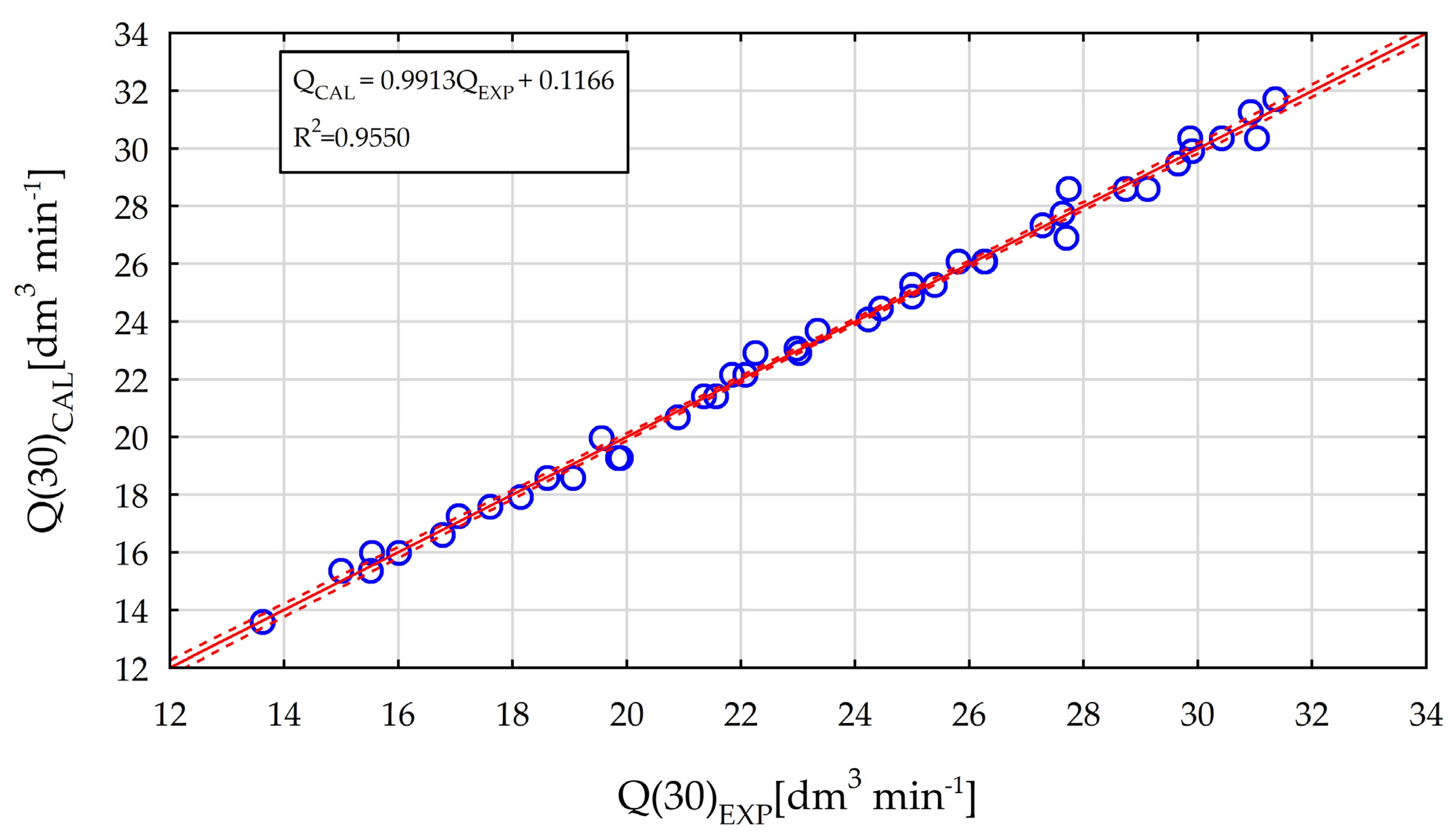
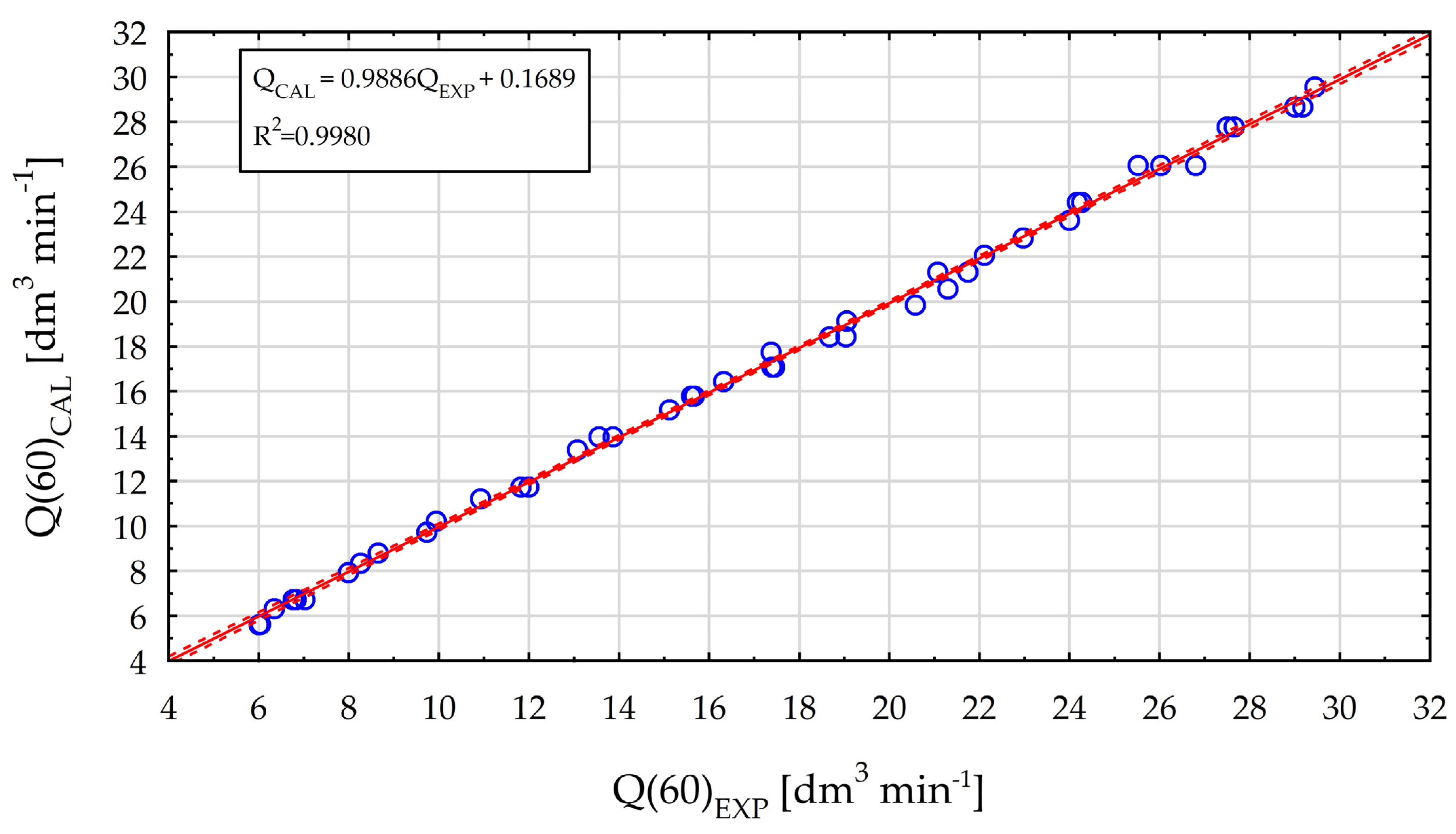
The least squares regression showed the strongest relationship between head and flow rate (R-squared = 0.9981) in the case of a slope of notch angle 45°. In the other cases, R-squared was also high, with values of R2 = 0.9955 and R2 = 0.9980, respectively (for the 30° and 60°). The smallest RMSE was 0.255 dm3∙min−1 for 44 flow rate calibration measurements (slope of crest angle 45°). In the other cases, the RMSE was higher by 36% and 30%, respectively (0.346 (30°) and 0.332 (60°) dm3∙min−1). Regression equations showing the relationship between measured (QREF) and calculated discharge (QCAL) were developed based on checked readings. These equations were shown in plots of dispersion (Figure 3, Figure 4 and Figure 5). The red color indicates a regression line with the 95% confidence interval marked with a red dotted line. Measured values were marked with blue circles. The literature on V-notch weirs does not clearly specify which angle is the most appropriate in this case. According to Shen [51], if the tip of the weir plate is thicker than 1/16 inch, the downstream edges of the notch should be chamfered to make an angle of not less than 45° with the surface of the crest. Prakash [52] tested weirs with similar chamfered crests, but they were additionally inclined. Herschy [53], in his chapter titled “Flow through weirs, flumes, orifices, sluices and pipes”, gave instructions on how to chamfer the downstream edge of the notch. According to his recommendation, this angle should not be less then 60°. The same suggestions were also made in the books by Bos [54] and Brassington [55]: “The V-notch weir should have a lip of between 1 mm and 2 mm and the downstream face should slope away from the lip at an angle of at least 60°”. Eli [56] also stated that this angle should be 60° ± 1° at ¼” (6.35 cm) thickness.
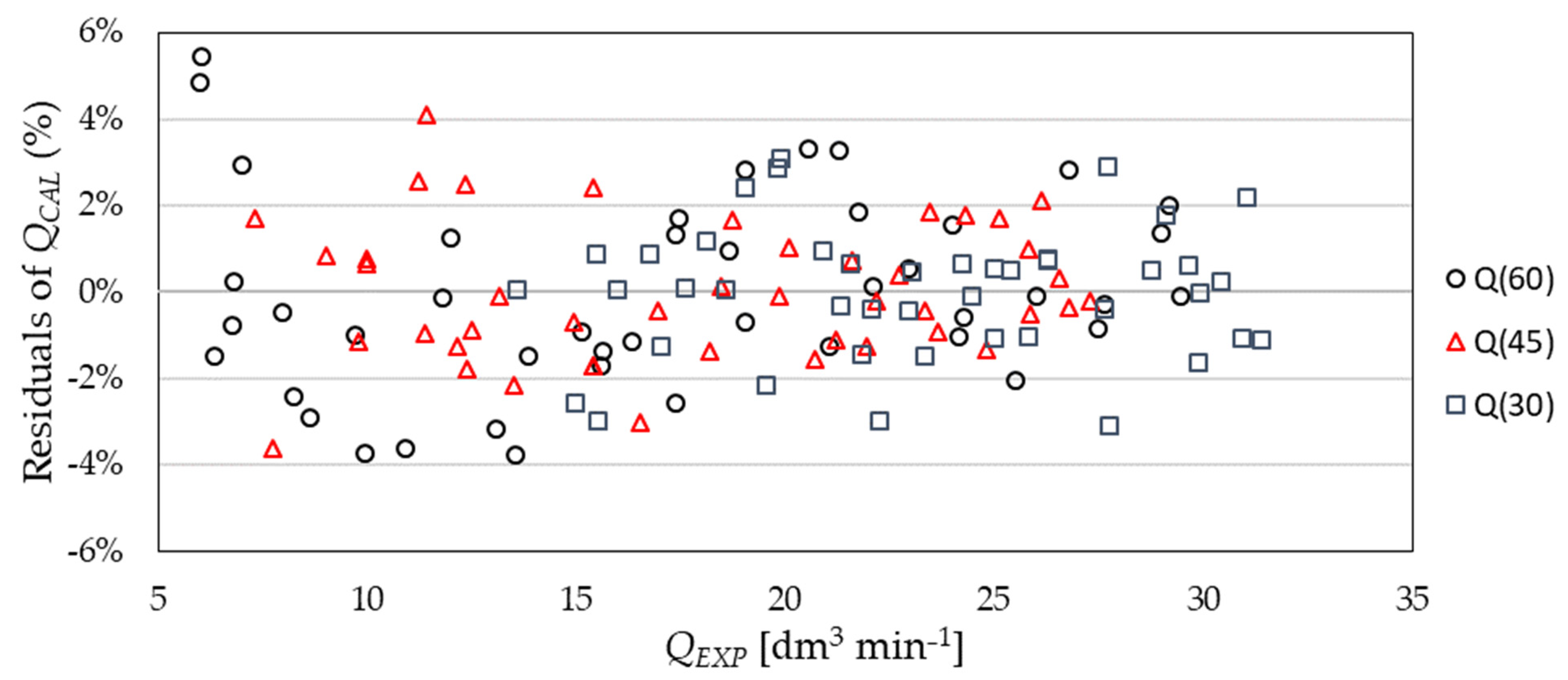
The conducted research shows that the use of a triangular weir with a chamfer of 30 degrees will require a greater height of the water table on the spillway for a proper outflow. In addition, it was observed during the tests that the stream was very unstable. The measured flow was susceptible to disturbances causing flow instability (e.g., the stream nappe stuck more easily to the walls of the overflow). In this research, a clear relationship was identified: with an increase of the chamfer angle of the spillway wall, the stream stabilized faster (Table 1). As a result, a larger chamfer angle gives a greater range of weir operation. Comparing the experimental QEXP and calculated discharges QCAL from the equations (Figure 3, Figure 4 and Figure 5), significant agreement is observed between calculated and measured discharges. Residuals of observed values versus calculated discharges were generally within the ±4% error limit and are acceptable (Figure 6). Taking into account the ranges of analyzed data, it seems that all the proposed equations predict discharges with high accuracy.
3.2. Comparison with Previously Reported V-Notch Weirs
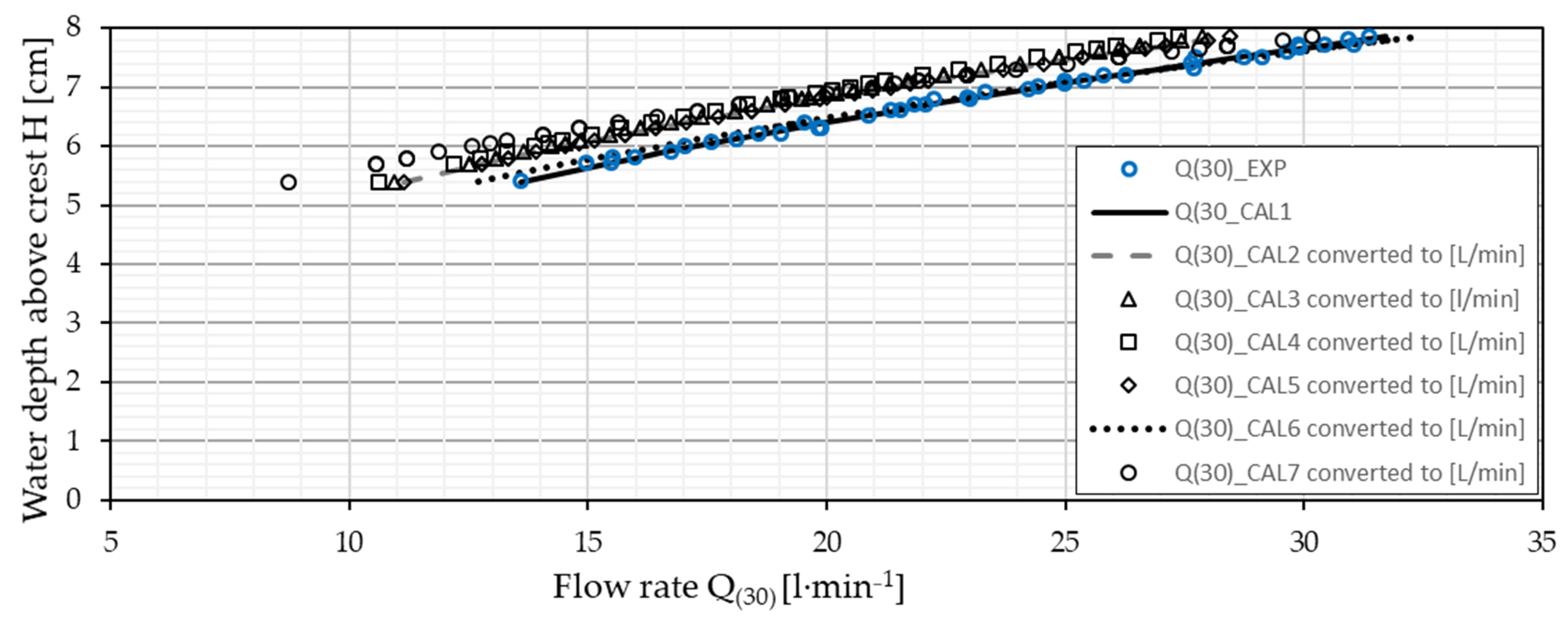
The obtained regression equations were compared with other studies conducted in agricultural and forest areas (Figure 7, Figure 8 and Figure 9). All of these studies focused on the issue of controlled drainage (CD).
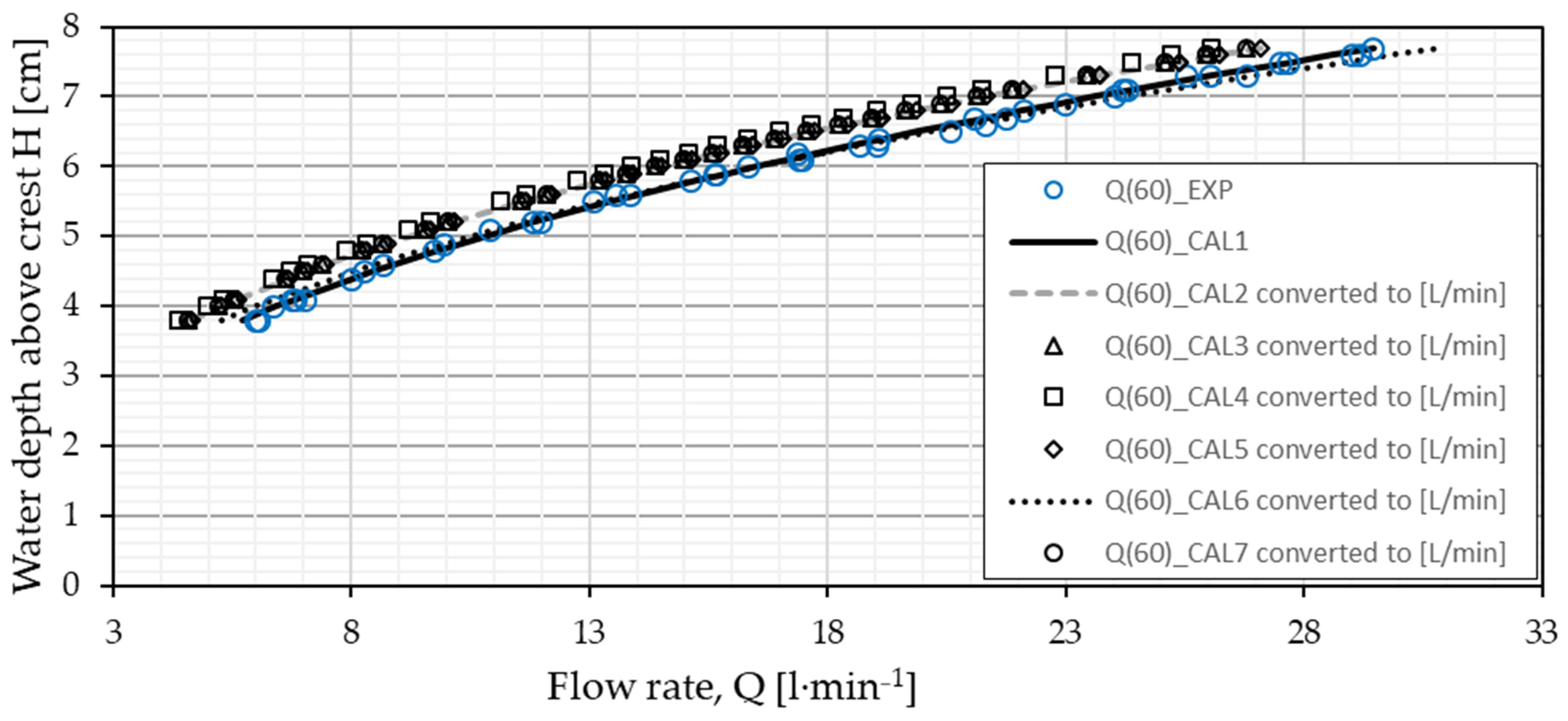
The analyses showed that only White’s equation [43], QCAL6, gave the best results of fitting to the empirical data for all the examined chamfered angles. However, the smallest measurement deviations were observed at the angle of 30° and 45°, and the largest at the angle of 60° (Figure 7, Figure 8 and Figure 9). This situation results from the fact that for the last analyzed variant, the height of operation of the V-notch when the nappe was stabilized, was the smallest. This is the moment when the measurement error is usually the greatest for all V-notch weirs. It should be noted that, according to the authors’ recommendations [46,47], the use of Formulas (4) and (5) requires the appropriate Cd to be maintained so that the overflows operate with full contraction. In the case of drainage wells, due to their small size, the installed V-notch weirs always operate with partial contraction. This means that the developed constant Cd indicators cannot be used in practice, and it is necessary to calibrate such weirs individually. Similarly, Shokrana and Ghane [39] claim, when using a cylindrical control structure, developing a step-discharge equation before monitoring drainage is recommended. According to the United States Bureau of Reclamation [48], the practical criterion for a partially contracted V-notch weir is H/B ≤ 0.4. The next equations describing the examined relationship reasonably well were Formulas (15) (QCAL2) and (3) (QCAL3). The QCAL2 equation is a formula that typically relates to an angle of 22.5°. It was used in studies including references [30,31,32,33,34]. In the case of the QCAL3 equation, a simplification of Cd = 0.44 was adopted for the entire measuring range. Interestingly, using a Cd of 0.578 [57] in the second Equation (2) would give virtually the same flow outcome. According to Shen [51], for h/p ratios higher than 0.16, the discharge coefficient is mainly a function of angle θ, and it is very stable with Re values. The performed analyses clearly show that the results of equations QCAL2 and QCAL3 for all analyzed angles are higher than the conducted measurements (Figure 7, Figure 8 and Figure 9). Also, in the case of Equations (16)—QCAL4 and (17)—QCAL5, the flow values are overestimated in relation to the measured data. It is important that for these equations, especially for angles of 45° and 60° (Figure 8 and Figure 9), the translation plot is proportional over the entire range of measurements. However, it should be borne in mind that Formula (16) from reference [10] uses a 15° V-notch weir. The last equation to compare the analysis (QCAL7) was taken from Formula (17). Although this formula applies to triangular weirs with a notch of 45°, the results obtained for the chamfer angle of 60° are very similar to formulas QCAL2, QCAL3, QCAL4, and QCAL5. These comparisons show how significant discrepancies appear in similar applications. They are also drawing attention to how important the slope of angle of the sharp-crested weir can be here.
4. Conclusions
In this study, the head and flow rate for a PC-edge sharp-crest 22.5° V-notch weir inside the fi400 cylindrical control structure were measured. Additionally, three different chamfered angles of the analyzed V-notch were investigated. Based on those measurements, the empirical stage-discharge equations were developed. In the calibration procedure, least squares methods were used. The empirical PC-edge sharp-crest 22.5° V-notch weir equations can be used for any cylindrical control structure, as long as the water is flowing through the V-notch weir and there is no flow submergence. In practice, using a tubular control structure is easier because of material availability and ease of construction. In conclusion, every V-notch weir equation developed in this study can provide reliable flow measurements that can be used to estimate nutrient load reductions in subsurface drainage studies. Nevertheless, the best results were achieved with a chamfer angle of 45°, and this would be the best choice.
Funding
This work was supported by the “Innovation Incubator 2.0” project financed from funds allocated for science as part of a non-competitive project implemented under the Smart Development Operational Program 2014-2020 (Poland), Priority Axis IV, no. MNiSW/2019/170/DIR.
Data Availability Statement
Not applicable.
Conflicts of Interest
The author declares no conflict of interest.
References
- Fowler, D.; Coyle, M.; Skiba, U.; Sutton, M.A.; Cape, J.N.; Reis, S.; Voss, M. The global nitrogen cycle in the twenty-first century. Philos. Trans. R. Soc. B Biol. Sci. 2013, 368, 20130164. [Google Scholar] [CrossRef] [PubMed]
- Galloway, J.N.; Townsend, A.R.; Erisman, J.W.; Bekunda, M.; Cai, Z.; Freney, J.R.; Sutton, M.A. Transformation of the nitrogen cycle: Recent trends, questions, and potential solutions. Science 2008, 320, 889–892. [Google Scholar] [CrossRef]
- Smith, V.H.; Tilman, G.D.; Nekola, J.C. Eutrophication: Impacts of excess nutrient inputs on freshwater, marine, and terrestrial ecosystems. Environ. Pollut. 1999, 100, 179–196. [Google Scholar] [CrossRef] [PubMed]
- Bissoli, R. Water Framework Directive 2000/60/EC. La Qual. Delle Acque Di Superf. 2008, 9–12. [Google Scholar]
- Carstensen, M.V.; Hashemi, F.; Hoffmann, C.C.; Zak, D.; Audet, J.; Kronvang, B. Efficiency of mitigation measures targeting nutrient losses from agricultural drainage systems: A review. AMBIO 2020, 49, 1820–1837. [Google Scholar] [CrossRef]
- Tournebize, J.; Chaumont, C.; Mander, Ü. Implications for constructed wetlands to mitigate nitrate and pesticide pollution in agricultural drained watersheds. Ecol. Eng. 2017, 103, 415–425. [Google Scholar] [CrossRef]
- Frankenberger, J.; Kladivko, E.; Sands, G.; Jaynes, D.; Fausey, N.; Helmers, M.; Cooke, R.; Strock, J.; Nelson, K.; Brown, L. Questions and Answers about the Drainage Water Management in the Midwest; Purdue Extension Publication (WQ–44): West Lafayette, IN, USA, 2006. [Google Scholar]
- Ale, S.; Bowling, L.C.; Owens, P.R.; Brouder, S.M.; Frankenberger, J.R. Development and application of a distributed modeling approach to assess the watershed-scale impact of drainage water management. Agric. Water Manag. 2012, 107, 23–33. [Google Scholar] [CrossRef]
- King, K.W.; Fausey, N.R.; Williams, M.R. Effect of subsurface drainage on streamflow in an agricultural headwater watershed. J. Hydrol. 2014, 519, 438–445. [Google Scholar] [CrossRef]
- Macrae, M.L.; English, M.C.; Schiff, S.L.; Stone, M. Intra-annual variability in the contribution of tile drains to basin discharge and phosphorus export in a first-order agricultural catchment. Agric. Water Manag. 2007, 92, 171–182. [Google Scholar] [CrossRef]
- Culley, J.L.B.; Bolton, E.F. Suspended Solids and Phosphorus Loads from a Clay Soil: II. Watershed Study; American Society of Agronomy, Crop Science Society of America, and Soil Science Society of America: Madison, WI, USA, 1983; Volume 12, pp. 498–503. [Google Scholar] [CrossRef]
- Xue, Y.; David, M.B.; Gentry, L.E.; Kovacic, D.A. Kinetics and Modeling of Dissolved Phosphorus Export from a Tile-Drained Agricultural Watershed; American Society of Agronomy, Crop Science Society of America, and Soil Science Society of America: Madison, WI, USA, 1998; Volume 27, pp. 917–922. [Google Scholar] [CrossRef]
- Edwards, I.J.; Jackon, W.D.; Fleming, P.M. Tipping bucket gauges for measuring run-off from experimental plots. Agric. Meteorol. 1974, 13, 189–201. [Google Scholar] [CrossRef]
- Lalonde, V.; Madramootoo, C.A.; Trenholm, L.; Broughton, R.S. Effects of controlled drainage on nitrate concentrations in subsurface drain discharge. Agric. Water Manag. 1996, 29, 187–199. [Google Scholar] [CrossRef]
- Wesström, I.; Messing, I.; Linner, H.; Lindström, J. Controlled drainage—Effects on drain outflow and water quality. Agric. Water Manag. 2001, 47, 85–100. [Google Scholar] [CrossRef]
- Wesström, I.; Joel, A.; Messing, I. Controlled drainage and subirrigation–A water management option to reduce non-point source pollution from agricultural land. Agric. Ecosyst. Environ. 2014, 198, 74–82. [Google Scholar] [CrossRef]
- Tait, R.; Madramootoo, C.A.; Enright, P. An instrumented, field-scale research facility for drainage and water quality studies. Comput. Electron. Agric. 1995, 12, 131–145. [Google Scholar] [CrossRef]
- Williams, M.R.; King, K.W.; Fausey, N.R. Drainage water management effects on tile discharge and water quality. Agric. Water Manag. 2015, 148, 43–51. [Google Scholar] [CrossRef]
- Ford, W.; King, K.; Williams, M.; Williams, J.; Fausey, N. Sensitivity analysis of the Agricultural Policy/Environmental eXtender (APEX) for phosphorus loads in tile-drained landscapes. J. Environ. Qual. 2015, 44, 1099–1110. [Google Scholar] [CrossRef]
- Nazari, S.; Ford, W.I.; King, K.W. Impact of flow pathway and source water connectivity on subsurface sediment and particulate phosphorus dynamics in tile-drained agroecosystems. Agric. Water Manag. 2022, 269, 107641. [Google Scholar] [CrossRef]
- Walkowiak, D.K. ISCO Open Channel Flow Measurement Handbook, 6th ed.; Teledyne ISCO, Incl.: Lincoln, NE, USA, 2008; pp. 132–142. ISBN 0-9622757-3-5. [Google Scholar]
- Szejba, D.; Bajkowski, S. Determination of tile drain discharge under variable hydraulic conditions. Water 2019, 11, 120. [Google Scholar] [CrossRef]
- Bajkowski, S.; Szejba, D. Adapter for Measuring Water Flow in Pipes. Patent Number PL396437-A1, 21 April 2015. [Google Scholar]
- Saadat, S.; Bowling, L.; Frankenberger, J.; Brooks, K. Effects of controlled drainage on water table recession rate. Trans. ASABE 2017, 60, 813. [Google Scholar] [CrossRef]
- Kolavani, F.L.; Bijankhan, M.; Di Stefano, C.; Ferro, V.; Mazdeh, A.M. Flow measurement using circular portable flume. Flow Meas. Instrum. 2018, 62, 76–83. [Google Scholar] [CrossRef]
- Bosch, D.D.; Potter, T.L.; Truman, C.C.; Bednarz, C.W.; Strickland, T.C. Surface runoff and lateral subsurface flow as a response to conservation tillage and soil-water conditions. Trans. ASAE 2005, 48, 2137–2144. [Google Scholar] [CrossRef]
- Allred, B.J.; Brown, L.C.; Fausey, N.R.; Cooper, R.L.; Clevenger, W.B.; Prill, G.L.; Czartoski, B.J. Water table management to enhance crop yields in a wetland reservoir subirrigation system. Appl. Eng. Agric. 2003, 19, 407. [Google Scholar] [CrossRef]
- Bos, M.G.; Repogle, J.; Clemmens, A.J. Flow Measuring Flumes for Open Channel Systems; Wiley-Interscience: New York, NY, USA, 1984; ISBN 0-471-80637-4. [Google Scholar]
- Bahceci, I.; Çakir, R.; Nacar, A.; Bahceci, P. Estimating the effect of controlled drainage on soil salinity and irrigation efficiency in the Harran Plain using SaltMod. Turk. J. Agric. For. 2008, 32, 101–109. [Google Scholar]
- Brooks, K. Measurement of Drain Flow, Soil Moisture, and Water Table to Assess Drainage Water Management. Master’s Thesis, Purdue University, Agricultural and Biological Engineering Department, West Lafayette, IN, USA, 2003. [Google Scholar]
- Sojka, M.; Kozłowski, M.; Kęsicka, B.; Wróżyński, R.; Stasik, R.; Napierała, M.; Jaskuła, J.; Liberacki, D. The Effect of Climate Change on Controlled Drainage Effectiveness in the Context of Groundwater Dynamics, Surface, and Drainage Outflows. Central-Western Poland Case Study. Agronomy 2020, 10, 625. [Google Scholar] [CrossRef]
- Liu, W.; Maxwell, B.; Birgand, F.; Youssef, M.; Chescheir, G.; Tian, S. Multipoint high-frequency sampling system to gain deeper insights on the fate of nitrate in artificially drained fields. J. Irrig. Drain. Eng. 2020, 146, 06019012. [Google Scholar] [CrossRef]
- Sunohara, M.D.; Gottschall, N.; Craiovan, E.; Wilkes, G.; Topp, E.; Frey, S.K.; Lapen, D.R. Controlling tile drainage during the growing season in Eastern Canada to reduce nitrogen, phosphorus, and bacteria loading to surface water. Agric. Water Manag. 2016, 178, 159–170. [Google Scholar] [CrossRef]
- Liu, Y.; Youssef, M.A.; Chescheir, G.M.; Appelboom, T.W.; Poole, C.A.; Arellano, C.; Skaggs, R.W. Effect of controlled drainage on nitrogen fate and transport for a subsurface drained grass field receiving liquid swine lagoon effluent. Agric. Water Manag. 2019, 217, 440–451. [Google Scholar] [CrossRef]
- Satchithanantham, S.; Ranjan, R.S.; Bullock, P. Protecting water quality using controlled drainage as an agricultural BMP for potato production. Trans. Asabe 2014, 57, 815–826. [Google Scholar] [CrossRef]
- Satchithanantham, S.; Ranjan, R.S.; Shewfelt, B. Effect of water table management and irrigation on potato yield. Trans. ASABE 2012, 55, 2175–2184. [Google Scholar] [CrossRef]
- Povilaitis, A.; Rudzianskaite, A.; Miseviciene, S.; Gasiunas, V.; Miseckaite, O.; Živatkauskiene, I. Efficiency of drainage practices for improving water quality in Lithuania. Trans. ASABE 2018, 61, 179–196. [Google Scholar] [CrossRef]
- Christianson, L.E.; Christianson, R.D.; Lipka, A.E.; Bailey, S.; Chandrasoma, J.; McCoy, C.; Cooke, R.A. Calibration of stainless steel-edged V-notch weir stop logs for water level control structures. Appl. Eng. Agric. 2019, 35, 745–749. [Google Scholar] [CrossRef]
- Shokrana, M.S.B.; Ghane, E. An empirical V-notch weir equation and standard procedure to accurately estimate drainage discharge. Appl. Eng. Agric. 2021, 37, 1097–1105. [Google Scholar] [CrossRef]
- Helmers, M.; Christianson, R.; Brenneman, G.; Lockett, D.; Pederson, C. Water table, drainage, and yield response to drainage water management in southeast Iowa. J. Soil Water Conserv. 2012, 67, 495–501. [Google Scholar] [CrossRef]
- Herschy, R. General purpose flow measurement equations for flumes and thin plate weirs. Flow Meas. Instrum. 1995, 6, 283–293. [Google Scholar] [CrossRef]
- Popek, Z.; Bajkowski, S.; Siwicki, P.; Urbański, J. Laboratory Tests of New Groundwater Table Level Regulators in Subsurface Drainage Systems. Water 2021, 13, 631. [Google Scholar] [CrossRef]
- White, F.M. Fluid Mechanics, 7th ed.; McGraw-Hill Companies, Inc.: New York, NY, USA, 2011; Available online: http://ftp.demec.ufpr.br/disciplinas/TM240/Marchi/Bibliografia/White_2011_7ed_Fluid-Mechanics.pdf (accessed on 3 August 2023)ISBN 978-0-07-352934-9.
- El Hattab, M.H.; Mijic, A.; Vernon, D. Optimised Triangular Weir Design for Assessing the Full-Scale Performance of Green Infrastructure. Water 2019, 11, 773. [Google Scholar] [CrossRef]
- Cording, A.; Hurley, S.; Whitney, D. Monitoring methods and designs for evaluating bioretention performance. J. Environ. Eng. 2017, 143, 05017006. [Google Scholar] [CrossRef]
- Kulin, G.; Compton, P.R. A Guide to Methods and Standards for the Measurement of Water Flow; US Department of Commerce, National Bureau of Standards: Washington, DC, USA, 1975; Volume 13. [Google Scholar]
- El-Ansary, M.Y.; Awad, M.A.; Nassar, A.A.; Farag, A.A. Calibration of three common flow measurement devices for open channels. Misr J. Agric. Eng. 2010, 27, 151–169. [Google Scholar] [CrossRef]
- USGS. Measurement and computation of streamflow. In Computation of Discharge (Geological Survey Water-Supply Paper 2175); USGS: Washington, DC, USA, 1982; Volume 2. [Google Scholar]
- ISO 1438:2017; Hydrometry—Open Channel Flow Measurement Using Thin-Plate Weirs. International Organization for Standardization (ISO): London, UK, 2017.
- Jaynes, D.B.; Isenhart, T.M. Reconnecting tile drainage to riparian buffer hydrology for enhanced nitrate removal. J. Environ. Qual. 2014, 43, 631–638. [Google Scholar] [CrossRef]
- Shen, J. Discharge Characteristics of Triangular-Notch Thin-Plate Weirs; (No. 1617); United States Department of the Interior, Geological Survey: Reston, VI, USA, 1981. [Google Scholar]
- Prakash, M.S.; Shivapur, A.V. Generalized head-discharge equation for flow over sharp-crested inclined inverted V-notch weir. J. Irrig. Drain. Eng. 2004, 130, 325–330. [Google Scholar] [CrossRef]
- Herschy, R.W. Flow through weirs, flumes, orifices, sluices and pipes. In Hydrology and Lakes. Encyclopedia of Earth Science; Springer: Dordrecht, The Netherlands, 1998. [Google Scholar] [CrossRef]
- Bos, M.G. (Ed.) Discharge Measurement Structures, 3rd ed.; ILRI Publication 20: Wageningen, The Netherlands, 1989; p. 320. [Google Scholar]
- Brassington, R. Field Hydrogeology; John Wiley & Sons: Hoboken, NJ, USA, 2023. [Google Scholar]
- Eli, R.N. V-notch weir calibration using new parameters. J. Hydraul. Eng. 1986, 112, 321–325. [Google Scholar] [CrossRef]
- Lenz, A.T. Viscosity and surface tension effects on V-notch weir coefficients. Trans. Am. Soc. Civ. Eng. 1943, 108, 759–782. [Google Scholar] [CrossRef]
Figure 1.
(a,b). Measuring flume with a new cylindrical control structure installed.

Figure 2.
Analyzed triangular weir: (a) front view of V-notch weir with angle of 22.5° and characteristic parameters, (b) different angles of downstream of the sharp edge: 30°, 45°, and 60°.
Figure 2.
Analyzed triangular weir: (a) front view of V-notch weir with angle of 22.5° and characteristic parameters, (b) different angles of downstream of the sharp edge: 30°, 45°, and 60°.

Figure 3.
Relationship between QEXP and QCAL by equation Q30 = 0.2977H2.2659.

Figure 4.
Relationship between QEXP and QCAL by equation Q45 = 0.2235H2.4182.

Figure 5.
Relationship between QEXP and QCAL by equation Q60 = 0.2564H2.3244.

Figure 6.
Percent residuals of QCAL vs. QEXP.

Figure 7.
Comparison of the V-notch equation discharge (Q30) determined in this study to the values in other studies.
Figure 7.
Comparison of the V-notch equation discharge (Q30) determined in this study to the values in other studies.

Figure 8.
Comparison of the V-notch equation discharge (Q45) determined in this study to the values in other studies.
Figure 8.
Comparison of the V-notch equation discharge (Q45) determined in this study to the values in other studies.

Figure 9.
Comparison of the V-notch equation discharge (Q60) determined in this study to the values in other studies.
Figure 9.
Comparison of the V-notch equation discharge (Q60) determined in this study to the values in other studies.


Table 1.
Simplification formulas of V-notch discharges for different slopes of crest angle.
| Angle of slope | Calculated Equation (QCAL1) | R-Squared (R2) | Root Mean Square Error (RMSE) | Height of Water above the Crest H (cm) (Range) | Range of Flow Measurement Q (L∙min−1) |
|---|---|---|---|---|---|
| 30° | Q = 0.298H2.266 | 0.9955 | 0.346 | 5.4–7.8 (2.45) | 13.60–31.38 |
| 45° | Q = 0.224H2.418 | 0.9981 | 0.255 | 4.2–7.3 (3.10) | 7.31–27.29 |
| 60° | Q = 0.256H2.325 | 0.9980 | 0.332 | 3.8–7.7 (3.90) | 6.00–29.45 |
Disclaimer/Publisher’s Note: The statements, opinions and data contained in all publications are solely those of the individual author(s) and contributor(s) and not of MDPI and/or the editor(s). MDPI and/or the editor(s) disclaim responsibility for any injury to people or property resulting from any ideas, methods, instructions or products referred to in the content. |
© 2023 by the author. Licensee MDPI, Basel, Switzerland. This article is an open access article distributed under the terms and conditions of the Creative Commons Attribution (CC BY) license (https://creativecommons.org/licenses/by/4.0/).
Share and Cite
MDPI and ACS Style
Napierała, M. Application of Simple Crested Weirs to Control Outflows from Tiles Drainage. Water 2023, 15, 3248. https://doi.org/10.3390/w15183248
AMA Style
Napierała M. Application of Simple Crested Weirs to Control Outflows from Tiles Drainage. Water. 2023; 15(18):3248. https://doi.org/10.3390/w15183248
Chicago/Turabian StyleNapierała, Michał. 2023. "Application of Simple Crested Weirs to Control Outflows from Tiles Drainage" Water 15, no. 18: 3248. https://doi.org/10.3390/w15183248
Note that from the first issue of 2016, this journal uses article numbers instead of page numbers. See further details here.