Article

Structural Connectivity of Asia’s Protected Areas Network: Identifying the Potential of Transboundary Conservation and Cost-Effective Zones

by
Melissa Penagos Gaviria
1,
Żaneta Kaszta
2,* and
Mohammad S. Farhadinia
3
1
School of Geography and the Environment, University of Oxford, Oxford OX1 3QY, UK
2
Wildlife Conservation Research Unit (WildCRU), Department of Zoology, University of Oxford, Tubney OX13 5QL, UK
3
Department of Zoology, Oxford Martin School, University of Oxford, 34 Broad Street, Oxford OX1 3BD, UK
*
Author to whom correspondence should be addressed.
ISPRS Int. J. Geo-Inf. 2022, 11(7), 408; https://doi.org/10.3390/ijgi11070408
Submission received: 25 April 2022 / Revised: 12 July 2022 / Accepted: 14 July 2022 / Published: 19 July 2022
(This article belongs to the Special Issue Geospatial Data and Services for Wildlife Management and Conservation)

Abstract

:
Human activities can degrade landscape connectivity and disrupt ecological flows, jeopardising the functional integrity of processes. This study presents a quantitative assessment of Asia’s protected areas’ (PAs) structural connectivity using landscape metrics, as well as analyses of the Cost-Effective Zones’ (CEZs). Using nine landscape metrics, we assessed connectivity at zonal (country borders and interior), national, regional, and geographical (islands and continent) levels. The results showed that the structural connectivity of Asia’s PAs network measured by a Connectance index was very low (0.08% without country borders and 9.06% for the average country analysis). In general, connectivity was higher within borders (0.36%) than within the countries (0.22%). Islands exhibited significantly higher Area-weighted mean patch area, Proximity index and Largest patch index, suggesting more integrity and connectiveness. When comparing Asian regions, Western Asia presented the lowest values for Percentage of landscape and Proximity index. We found that only 15% of the CEZs in Asia were under PAs designation, and more CEZs are located in the interior, but the majority with the highest priority was in the borders (9%). We advocate that expanding PAs coverage, specifically targeting areas that increase connectivity (e.g., through transboundary PAs), should be a priority to maintain their ecological function.

1. Introduction

Global biodiversity is decreasing faster than at any time in human history [1]. The levels of biodiversity loss have brought to light the need for international collaboration and cooperation for the protection of nature [2]. In 1992, the Convention of Biological Diversity (CBD) was created, aiming for the conservation of biological diversity, the sustainable use of its components, and the fair and equitable sharing of the benefits [3]. The CBD adopted “Aichi Targets” to address and reduce the causes of biodiversity loss, and to promote sustainable usage by 2020. Specifically, Target 11 stated that “At least 17 per cent of terrestrial and inland water, is conserved effectively and equitably managed, is ecologically representative and well-connected systems of protected areas and other effective area-based conservation measures” for 2020 [4]. This resulted in the rapid expansion of the global network of protected areas (PAs). Yet the target was only partially achieved [5], as PAs currently cover approximately 15% of the terrestrial surface [6]. Furthermore, the new Global Biodiversity Framework is being negotiated, which aims at protecting at least 30% of the world’s land and ocean by 2030 [7].
However, this Target was not merely a spatial coverage metric but also included qualitative features, such as “well-connected” PAs. Despite the moderate progress in reaching PAs’ area target, PAs connectivity remains far from being achieved. A global assessment indicated an expansion of protected connected land from 6.5% in 2010 to 7.7% in 2018 [8]. A higher emphasis on planning to reconnect habitat patches or preserve existing connectivity is required [9].
Ecological processes and species ranges are rarely coincident with socio-political borders, nor are the environmental issues and conservation challenges surrounding conservation planning [10,11]. Political borders generate important conservation implications as they fragment policy and legislation across species ranges [12]. Additionally, due to climate change, the ranges of many species are likely to shift across international borders [10,13]. There is, therefore, a strong need to identify key habitats to prioritize conservation efforts, accounting for the effects of political borders. Hence, some areas have been identified as Cost-Effective Zones (CEZs) based on global biodiversity prioritization templates that are extensively recognized and located in areas of low human impact [14,15]. Yet, large areas of CEZs are globally unprotected [14], not achieving the representation target.
The Asian continent accounts for almost a third of the world’s land, yet only around 13.5% of Asia is protected [6]. Moreover, it contains approximately 82% of global border hotspots for threatened transboundary species [11]. For instance, the Middle East has been highlighted as an area with high wildlife transboundary movement relative to its species richness [16]. Although the global distribution of threatened species with transboundary ranges is concentrated primarily in Southeast Asia [11], most work on the development and implementation of transboundary protected areas (TBPAs) has been conducted in Europe, Africa, and America [10,17,18]. In Asia, PAs tend to be located close to international borders [19,20], suggesting a greater potential in Asia for PAs structural connectivity across countries borders [20]. Furthermore, Asia was the only continent with lower connectivity in 2018 than in 2010, decreasing from 6.2% to 5.1% in 2018 [8], highlighting the urgent need to evaluate the current state of connectivity and to establish alternatives to reach the target.
In this study, we evaluated the structural connectivity of the Asian terrestrial PAs system, at zonal (country borders and country interior), national, regional, and geographical (islands and continent) levels using nine landscape metrics. We also assessed the representation of CEZs in the current level of protection. The following hypotheses were tested: (1) There is greater structural connectivity between PAs across international borders than PAs within the interior of Asian countries [19,20,21]; (2) PAs in Asian islands are more connected than the continental PAs; (3) the distribution and the PAs designation of CEZs is higher in borders than within the countries [14,22].
There is an urgent need to define where to designate new PAs or expand the existing ones to boost their effectiveness and feasibility, with a primary goal to increase PAs connectivity. This study aims to facilitate evidence-based decision-making for PAs designation at a continental level targeting PAs network connectivity, and integrating Cost-Effective Zones in the prioritization process. Hence, this work can help to identify priorities and potential for international cooperation towards achieving the targets of the post-2020 Global Biodiversity Framework for maintaining ecological landscape connectivity.

2. Materials and Methods

2.1. Study Area

The study area covered all Asian countries. Similarly to Kamath (2020) [20], countries with their territories both in Asia and Europe, including Armenia, Azerbaijan, Georgia, Kazakhstan, Russia, and Turkey, were included in the analyses. Island countries without a land border with another country, like Sri Lanka and Bahrain, were excluded, as the study aimed to compare terrestrial connectivity. The whole studied region stretches over an area of approximately 502.5 million km2 (Figure 1).
The countries were grouped into regions according to United Nations’ geographical regions classification [23], adding the Caucasus region which included Georgia, Azerbaijan, and Armenia. For the countries outside Asia, the regional name corresponded to the continent, including “Europe” and “Africa,” as their specific region is not required for the continental analysis. Thus, the regions included were Eastern Asia, Southern Asia, Central Asia, Southeastern Asia, Western Asia, Russia, Caucasus, Africa, and Europe. Regions were analysed as they represent a broader scale for decision making and as country borders are human created but not necessarily natural boundaries. Hence, landscape actions can be more efficient. Whilst there are different methods to define geographic areas, such as ecoregions, there are substantial distribution differences according to each proposed scheme. Besides, the insufficiently detailed data at large geographic scales have hindered the progress in refining biogeographical regions [24]. Furthermore, regional partnerships and coordinated actions are usually made on an economic and political basis, rather than on ecological priorities. A list of countries and territories classified into regions are provided in Appendix A, Table A1.

2.2. Protected Areas
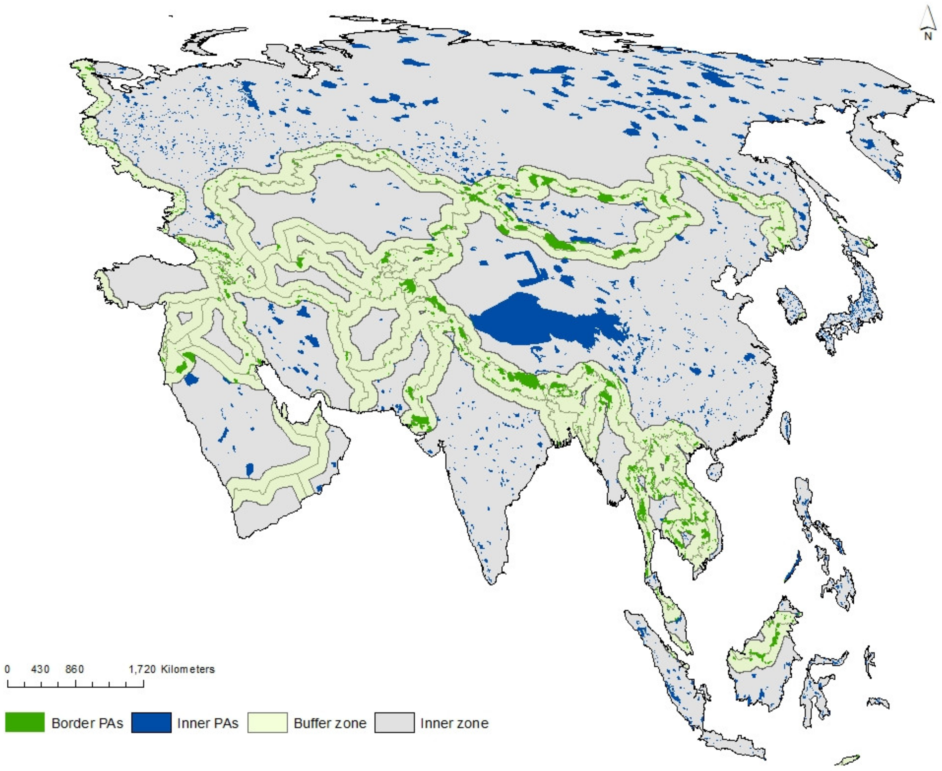
The 2020 World Database of Protected Areas (WDPA) was used for these analyses [25]. Due to the removal of most of China’s PA from the public May 2019 WDPA version, the WDPA Chinese data from 2017 were used for the analyses. We used PAs listed under the International Union for Conservation of Nature (IUCN) categories 1–6, which includes PAs with strict conservation aims to the ones that allow sustainable use of the landscape. It is acknowledged that some PAs may have been created since then and are not updated, and that some are not reported. Additionally, neither the existence nor the typology of PAs can ensure effective management and conservation. PAs with ‘Not Reported’ and ‘Proposed’ status were excluded from the analyses. Only terrestrial PAs were included. The same above-mentioned filters were applied to China’s PAs. North Korea was excluded from our analyses due to the lack of data on PAs.
The WDPA dataset contains overlapping PAs polygons with variances in the designation categories. To avoid double-counting, we dissolved the layer [26] to aggregate overlapping polygons. These resulted in a total of 40,380 PAs. The layer was projected to WGS_1984_Eckert_IV, which is an equal-area projection which are used when comparing areas or estimating the number of features per area unit and that has very low mean angular distortion [27,28]. Based on this layer, we produced several rasters of 700 × 700 m resolution used for all subsequent analyses.

2.3. Zones

In this study, a border refers to the politically established geographic boundaries of a nation, and transboundary PAs are the ones located across international boundaries within a predefined 125 km buffer from these boundaries. The buffer was determined based on the results of Thornton et al. (2020) [21] and Kamath (2020) [20] studies, who reported a declining trend in the proportion of PAs away from the border, up to 125 km. In addition, buffer areas were generated for no Asian countries that share boundaries with Asia.
For landlocked countries, an internal buffer was generated. For Asian countries with coastlines, an external buffer was applied to the borders of all the adjacent countries, avoiding the creation of a buffer in the coastline area that does not share borders with other countries.
To represent the interior country zones, a layer excluding the buffered boundary area was created. The PAs dataset was clipped to the buffer (hereafter referred to as ‘a border layer’) and to the layer excluding the buffer (hereafter referred to as ‘an internal layer’).
We then generated the layers, corresponding to the general, border, and internal level. Each of them was produced distinguishing and without distinguishing the countries.
After creating the 125 km buffer from the country’s borders, 72% of the study area corresponded to the “internal”, and 28% to “the border” zones. The study area was also classified according to the geographical classification, between “continent” and “islands” using the intersect tool.
The statistical analyses described below were carried out separately for each layer.

2.4. Connectivity Analyses

The structural connectivity of the Asian PAs network was calculated using FRAGSTATS v4.2.1 [29]. FRAGSTATS is a spatial pattern analysis software designed to quantify the structure (i.e., composition and configuration) of landscapes by including more than 80 different metrics [30], and thus the software is the most comprehensive tool to measure the structural landscape connectivity.
We selected nine different landscape metrics, which can best measure and quantify the connectivity of our study area at various levels: (1) Percentage of landscape (PLAND), (2) Distribution of patch area (AREA_AM), (3) Patch radius of gyration (GYRATE_AM), (4) Edge density (ED), (5) Landscape Patch index (LPI), (6) Patch density (PD), (7) Number of patches (NP), (8) Connectance index (CONNECT), and (9) Proximity index (PROX) (Table 1). CONNECT and PROX were analysed at three different radiuses: 10, 20, and 30 km. These values were selected in relation to the median dispersal abilities of the large majority of terrestrial species [31]. Shapiro Wilk test was used to evaluate the normality in the distribution of residuals.
To mitigate the limitations of isolation metrics, which use the nearest-neighbour distances that are calculated from patches within the landscape boundary [30], we used different thresholds/scales for these metrics. Furthermore, PROX was created to address this constraint, and it takes into consideration the size and proximity of all patches whose edges are in a set search radius of the focal patch [30].
The connectivity analysis was performed at four levels: (1) zonal, (2) geographic classification, (3) countries, and (4) regional analyses. The zonal analysis referred to a comparison between border and countries’ internal areas, based on the 125 km buffer. The geographical classification analysis evaluated the difference between the Asian islands and the continental Asia. Additionally, a set of comparisons between countries and regions were done.
As the data were not normally distributed, we used a non-parametric Wilcoxon signed-rank test to evaluate the differences at zonal (between internal and border zones) and geographical scales (between islands and continental areas). Kruskal-Wallis test by rank was used to evaluate regional categories. The statistical tests were done in R v 1.3 [32].

2.5. Cost-Effective Zones (CEZs) Assessment

The CEZs identified by Yang et al. (2020) were used to determine the distribution of the CEZs between the study zones and to analyse their coverage by the existing PAs network [33]. The analyses can serve to determine current gaps and the priority of cost-effective areas for future establishment.
Following Yang et al. [33], we defined Conservation Priority Zones (CPZs) by overlaying nine different schemes, including Key Biodiversity Areas [34], Crisis Ecoregions [35], Biodiversity Hotspots [36], Endemic Bird Areas [37], Key Biodiversity Areas [38], Centres of Plant Diversity [39], Global 200 Ecoregions [40], and Intact Forest Landscapes [33,41] (Figure 2). Secondly, these areas were classified into three categories: level 1 conservation priority zones (CPZs) representing areas covered by three or more templates; level 2 CPZs for those under two templates; and level 3 CPZs for the ones covered only by one scheme [33]. Subsequently, the Low Impact Areas [42] layer was overlaid to identify CPZs under low levels of human impact further called Cost-effective Zones (CEZs) [33]. Thus, CEZ1 were areas with three or more templates in Low Impact Areas, CEZ2 the ones with two schemes in Low Impact Areas, and CEZ3 the ones with one template and Low Impact Areas.
Areas and proportions were calculated using the Zonal statistics [26]. We calculated the proportion of each CEZs type in each zone in relation to the total area was calculated (CEZs type by zone/CEZs total area), the proportion of each CEZs type in each zone with each zone area (CEZs type by zone/zone area), and the relation of each CEZs type with the area of each CEZ type (CEZs type by zone/total CEZs type area). After testing normal distribution with the Shapiro Wilk test, an unpaired two-samples t-test was used to compare zones (internal and border), and an ANOVA test to compare the different levels of CEZs.

3. Results

3.1. Zonal Analysis: Internal vs. Border Zones

The amount of terrestrial land designated as PAs in border zones doubled the PAs in the internal area (7.6% and 3.5%, respectively). Different results were found when including countries or when analysing the region without distinguishing countries, although the CONNECT metric was greater in borders than in the internal zone in both analyses.
At a regional level, without including country borders, all the connectivity metrics had higher values in the internal zone except for the CONNECT metric, which was higher in borders. The CONNECT metric for border zones was greater than the countries’ internal zones at all 3 radiuses (10 km internal: 0.06 vs. border: 0.09%; 20 km internal: 0.13% vs. border: 0.22%; and 30 km internal: 0.22% vs. border: 0.36%). PLAND, NP, PD, LPI, ED, AREA_AM, and GYRATE_AM presented higher values in the internal zone (Appendix B, Table A2).
In contrast, at a countries level, GYRATE_AM, CONNECT, and AREA_AM significantly differed between borders and the internal zone. The mean of the AREA_AM metric was significantly higher in the internal zone than in borders (internal: 1,465,461 ha; border = 432,202 ha, p = 0.048) (Figure 3A). In contrast, GYRATE_AM, representing the distance between each cell within the patch and the patch centroid, was higher in the borders than in the internal area (internal: 21 km; border: 24 km, p < 0.014) (Figure 3B). There was also a significant difference in the PAs’ CONNECT metric between the internal and border zone (p = 0.011, p = 0.018, p = 0.23, respectively) across all evaluated radiuses (10, 20, and 30 km) (Figure 3G). The CONNECT metrics for border zones were twice or more than the results in the internal zones. The lowest CONNECT result was 3.06% for internal areas at a 10 km radius, and 11.58% was the highest result, found at 30 km radius in the border area. The other metrics means were not significantly different between the borders and the internal areas within countries’ boundaries (p > 0.05).

3.2. Geographical Classification Analysis: Islands vs. Continent

Islands represented 5.6% of the study area, whereas continental landmass represented 94.4%. LPI (continent: 0.05%; island: 0.14%, p < 0.001), ED (continent: 0.002 vs. island: 0.03, p < 0.001), and the PLAND (continental: 0.15% vs. island 0.64%, p = 0.002) of PAs were significantly higher for islands (Figure 3C,D,F). For the aggregation metrics, PD also exhibited significantly higher levels for islands (p = 0.0012) (Appendix C, Figure A1).
In general, at the country level, the highest PA’s PROX and LPI were found in the internal islands zone (Figure 3D). However, at the continental level, PROX was higher in the border zone (Figure 3H). At a country level, there was no evidence for a difference in the CONNECT across different radius thresholds between continent and island borders (p > 0.05; Figure 3G).

3.3. Regional Analysis

Several connectivity metrics (PLAND, NP, ED, LPI, and PROX for the 3 radiuses) showed significant differences between the regions (Figure 4). Eastern Asia had a significantly higher PLAND mean (0.7%) compared to Central (mean: 0.03%, p = 0.015), Southern (mean: 0.06%, p = 0.015), Southeastern (0.35%, p = 0.043) and Western Asia (0.02%, p = 0.004). In contrast, Western Asia had the lowest PLAND of PAs (mean: 0.02%), being also significantly lower compared to Southeastern (p = 0.009), and Russia (p = 0.037) (Figure 4A).
Eastern Asia showed the highest NP in the region (mean: 530.3, p < 0.05), significantly different to Central, Southeastern, Southern, and Western Asia (Figure 4C). ED in Eastern Asia (mean: 0.035, m/ha, p < 0.05) was higher than ED in Caucasus, Central, Southern, and Western Asia. Russian ED (mean 0.01 m/ha, p < 0.05) also was significantly higher than in Southern Asia (Figure 4B). Eastern Asia exhibited a significant higher LPI (mean: 0.26%, p < 0.05) than Central, Southern, and Western Asia (Figure 4D).
Western Asia exhibited a significantly lower PROX mean (~2.9, p < 0.05) than Eastern Asia (~182.4) for the 3 radiuses. Eastern Asia and the Caucasus were the regions with the highest PROX mean (182 and 96.3 respectively) (Figure 4E,F).

3.4. Country-Level Analysis

In general, the average connectivity of Asian countries was 8.85% (CONNECT was 6.49%, 8.89%, and 11.16% for 10, 20, and 30 km thresholds, respectively). On a national scale, the highest CONNECT levels were found in Bhutan, Lebanon, and Brunei Darussalam (Figure 5G). Kyrgyzstan was the country with the highest CONNECT metric in the internal zone, whereas for most of the countries (77.5%) it was higher in borders. Most of the countries showed low levels of structural connectivity (Figure 6). Only five countries (12.5%) presented a >10% CONNECT for the 10 km threshold for the general layer, and when using the 30 km radius, only five countries (12.5%) countries had >30% CONNECT. Additionally, 40% of the countries had a 0–2% CONNECT index at 30 km (Figure 5G).
Bhutan also exhibited the highest PROX (mean for the 3 radiuses: 4079), as well as China (mean: 1248) and Thailand (mean: 545). Notably, the PROX for the Philippines in the country’s internal area is among the five highest, but the border one is amongst the lowest values (internal: 167; border: 0). Low values of PROX were also found in Afghanistan and the United Arab Emirates (Figure 5H).
China’s internal zone had the highest level of GYRATE_AM (343.7 km), ten times higher than the median for all the countries (34 km) (Figure 5A). China also had a higher LPI (1.6%) in comparison with other countries (median: 0.05%). Bhutan (75.3 km), Myanmar (66.8 km), and Tajikistan (56.9 km) also had a high GYRATE_AM, specifically in their border zone (Figure 5E).
Over 25% of the total PAs’ PLAND in Asia is comprised of five countries (Indonesia, China, Japan, Russian Federation, and the Philippines), mainly from their internal area (Figure 5D). Japan, Indonesia, and South Korea had the highest levels of both ED (0.23 m/ha, 0.1 m/ha, 0.08 m/ha respectively) (Figure 5C) and PD (0.001, 0.0001, 0.0006 number per 100 ha, respectively). In contrast, Lebanon and Qatar revealed the lowest levels for ED, PD, LPI, and PLAND (0 value), besides AREA_AM (147 ha, 98 ha, respectively). The highest AREA_AM was found in China, Myanmar, Tajikistan, and Bhutan (Figure 5B); while 70% of the total NP corresponded to Japan, South Korea, and Russian Federation (Figure 5F).

3.5. Cost-Effective Zones (CEZs) Assessment by Zones

On average, over one-third of the study area corresponded to any of the three CEZs levels (internal: 26.5% and border: 8.99%). The coverage of the CEZs in relation to the area of each study zone was similar (internal: 37.4%, border: 30.76%, proportionally to each zone area). However, only 15.04% of the CEZs within the study area (internal: 10.7%, border: 4.4%) were under PAs designation. When looking at the CEZs under PAs designation within the border and country interior calculated as a proportion of the entire area under CEZs, we did not find any significant differences between border and interior zones (inner: 18.1%, border: 17.4% average, p > 0.05).
The CEZ3 represented over half of the proposed CEZ (57.9%), and 82.8% of the CEZ3 were in the internal zone of the countries. However, only 10.5% of the CEZ3 were under PAs protection in the study area. CEZ1 presented the highest PAs designation (23.5%) when analysed proportionally to its area of coverage.
When analyzing each CEZs type with the total CEZs area, there was an almost equal proportion of CEZ1 in the borders and internal zone (border: 8.98%, internal: 8.47%). In contrast, CEZ2 (internal: 18.29% and border: 6.32%) and CEZ3 (internal: 48.0%, border: 9.95%) were higher in the countries interior than in the border zones. Yet, when comparing each CEZs type with the area of each study zone, CEZ1 in borders doubled the CEZ1 in the internal zone (internal: 4.24% and border: 10.94%); the contrary to what was found with CEZ3 (internal: 24.03% and border: 12.12%). CEZ2 was similar in both zones (internal: 9.16% and border: 7.70%).

4. Discussion

Our study showed that most of the PAs in Asia were not structurally connected. Yet, higher levels of connectivity were detected when comparing countries border zone with their interior areas. Moreover, areas of ecological priority do not appear to be targeted and designated as PAs, as the coverage of Cost-Effective Zones by PAs in Asia was low. These areas represent an opportunity for expansion of the PAs network, and thus increasing habitat connectivity for wildlife in Asia.

4.1. Internal vs. Countries’ Border Zones

We found a significantly higher density of PAs located along borders than in the internal zone, which confirms the “high and far” PAs paradigm, in which PAs tend to be distributed in areas distanced from big population centres and in high altitudes [22]. The higher structural connectivity across border zones could be associated with higher levels of connectivity between the PAs within the tested radiuses.
The higher density of PAs and higher structural connectivity in the border zones provide an insight into the potential of coordinated action to increase connectivity in the region. Fostering a collaborative conservation effort permits the identification of priority areas at a bigger scale. It constitutes an opportunity to efficiently use economic resources. For instance, the study of both the cost of conservation and threats to biodiversity in the Mediterranean Basin showed that a fully coordinated conservation plan in the Mediterranean Basin could save 45% of the total cost of an uncoordinated plan [43]. Similarly, Allan et al. (2019) found that a collaborative conservation approach in the Nile River would save 34% of the costs [44]. Nonetheless, large-scale plans and designation of TBPAs could also imply an increment in transaction costs and time due to more complex communication and management needs because of different languages, cultures, religions, political agendas, governance, and institutions, and could potentially disadvantage local communities [43,45]. Hence, TBPAs mechanism is recommended to be regarded as a potential management strategy being adapted to each particular context, not as an absolute effective strategy [46]. The success of the regional collaboration is also dependent on the inclusion of local strategies and agendas, less centralized and more integrated into the local context [17,47].

4.2. Zonal-Level Connectivity: Islands vs. Continent

Islands had higher PAs coverage percentage, higher integrity and connectiveness among relatively extensive PAs and less isolation than the continental Asia. Mouillot et al., 2020 also reported that PAs coverage on islands is higher than global coverage, although there was a lot of variation between islands. The heterogeneity of protection coverage among islands might be associated with climate, language diversity, human population density, and development [48].
Most of the islands from the study area occurred in the Malay Archipelago (Maritime Southeast Asia). Brunei Darussalam was the island with the highest structural connectivity, while Indonesia had the highest levels of connectivity and thus high conservation potential. Parts of this region are already protected by The Heart of Borneo, which represents an example of transboundary conservation between Brunei Darussalam, Indonesia, and Malaysia established in 2007 [49]. The initiative has the potential to limit further forest fragmentation and restore the connectivity of PAs, although its effectiveness has been questioned due to fragile governance, insufficient transboundary collaboration, and development projects such as infrastructure and agriculture [50]. Yet, the high levels of structural connectivity suggest that this transnational conservation effort could have played a role in effectively maintaining the connectivity in Borneo.

4.3. Regional and Country-Level Connectivity

We found that in general only 9.06% of the PAs were structurally connected across Asia. Extremely low levels of landscape connectivity between PAs in Asia (five times lower than connectivity in Oceania and the Americas [51]) have been also previously reported by Ward et al. (2020) and Saura et al. (2019) reporting approximately 5.2% PAs connectivity in Asia in 2018 [8]. However, it is not possible to numerically compare it to our results since the authors applied different methodologies and metrics to calculate connectivity. Our findings showed that Western Asia had the lowest coverage of PAs and high levels of PA isolation. In contrast, Eastern Asia showed the highest level of PAs coverage and cluster of larger patches, which is related to the high values presented in Japan and China. Central Asia exhibited some of the lowest number of PAs, with high levels of isolation. Although Russia presented the highest PAs coverage, connectivity levels were relatively low. Santini et al. (2016) reported that the PAs of the larger countries in Asia had very low connectivity, unlike smaller Asian countries [52]. The high number and percentage of area covered by PAs in Southeastern Asia were related to the number of PAs in Indonesia, whereas proximity values presented a high variation between the countries of this region, being high in most of the countries such as Thailand, Cambodia, the Philippines, Indonesia, and Malaysia, but very low in Timor-Leste. Low isolation level was also evident in the Caucasus, a region listed as a biodiversity hotspot [53], but also considered an ‘ecological island’ [36]. All this highlights the opportunity for collaborative conservation action in a landscape and regional level and the importance of improving connectivity at a continental level.
The percentage of structurally connected PAs presented high variability across Asian countries. For instance, Bhutan showed the highest structural connectivity and proximity of the PAs and the lowest fragmentation. As mandated in its constitution, at least 60% of the country should remain under forest cover [54] and almost 50% of Bhutan’s territory is designated as PAs [55].
Our analyses revealed that China had high proximity between PAs and a low level of fragmentation. Similarly, neighbouring Myanmar also exhibited a low level of fragmentation and high levels of habitat continuity between the PAs, indicating an extensive and highly traversable network of PAs between the two countries. China’s PAs network is reported to have a potentially important role in continental structural connectivity, yet the current, yet further attempts to increase the connectivity of Chinese PA’s with neighbouring countries are desirable [52]. For instance, for species such as the giant spiny frog (Quasipaa spinosa), improving the connectivity in southern China and the Sino-Vietnamese can represent critical refugia [56].
In West Asia, Lebanon and Qatar had the lowest coverage of PAs in their territory whereas Saudi Arabia, United Arab Emirates, Iraq, and Qatar had a PROX index of zero indicating high levels of PA isolation at the tested radiuses. Interestingly, although Lebanon had only 2.18% of its territory protected with a small number of PAs, our analyses showed that the country’s PAs scored high in the structural connectivity.

4.4. Cost-Effective Zones (CEZs)

In general, there was a low proportion of CEZs under PAs protection (~15%), suggesting that there are still many priority areas that yet need to be protected. The schemes used to classify the CEZs aimed to prioritize limited conservation funding [57], not specifically to recommend areas for PAs establishment [58]. In 2012, an analysis of PAs coverage reported that despite the increase of PAs area, the rate of PAs covering priority zones (Important Bird Areas and Alliance for Zero Extinction sites), drastically declined since 1950, implying that PAs were not being created in the important sites for species conservation [59].
Our findings showed that the majority of CEZ3 areas, representing areas covered by one global biodiversity template (i.e., key biodiversity areas) and identified as ‘Low human impact area’, were located in the internal zone. This type of CEZs also had the lowest level of PAs coverage. In contrast, most of CEZ1 areas, corresponding to the highest priority for biodiversity conservation areas which are covered by three or more global biodiversity templates identified as ‘Low human impact area’, were located in the border zones, especially when evaluating it in relation to the area of each study zone. The high number of CEZ1 can be related to the fact that around 82% of worldwide border hotspots for vulnerable transboundary species, notably the richest 5% of border segments, were found in Asia [11]. Although CEZ1 presented the highest PAs coverage when analysed proportionally to its area of coverage, its designation is still low. Thus, understanding the need and the goal of expanding the global PAs, borders represent a higher opportunity of creating or expanding PAs in the areas of the highest priority for biodiversity conservation.
Combining CEZs with connectivity measures offers a possibility to identify areas of high ecological importance with a lower investment cost, which also increases PAs connectivity, for example, through establishing TBPAs.

4.5. Conservation Implications

In this section, we seek to provide some insights that go beyond the research metrics and that might facilitate decision-making for conservation management.
Despite the expansion of the coverage of PAs, the state of the connectivity component of Aichi target 11 remains unclear and lacks a quantifiable target without any specific indicator [60]. Insufficient capacity in science, cooperation, legislation, and monitoring also limits its implementation [61]. The post-2020 Global Biodiversity Framework should include more clear, flexible, ambitious goals with defined pathways to reach them which is currently limited to only 8.85% of the Asian PAs as structurally connected.
Our spatial analysis demonstrated the low coverage of CEZs by PAs in Asia, implying that PAs tended to be located in the less important sites for species conservation [59]. This highlights the need for better placement/expansion of future PAs. Importantly, other effective area-based conservation measures [62], defined as “geographically defined areas other than PAs, governed to achieve positive biodiversity conservation outcomes with associated ecosystem functions and services as well as cultural, spiritual, socio-economic, and other locally relevant values” [51], can provide the opportunity to ensure wider connectivity is achieved through targeting towards ecologically priority areas. Furthermore, even if PAs have not been located in high-priority areas, maintaining their connectivity is a key aspect to maintain populations as their range shifts, considering land-use changes and climate change scenarios.
The infrastructure development plans in the region, such as the Belt and Road Initiative (BRI), represent a challenge towards the maintenance of the existing landscape connectivity, which is already low at the continental level. As one of the largest infrastructure projects in the world, BRI includes 71 countries [63], and seeks to promote the economic connectivity of Asian, European, and African continents. Roads and railways are a direct cause of landscape fragmentation, a rise in wildlife mortality, displacement, habitat degradation, and population dynamics alteration [64], [65]. For instance, Kaszta et al. (2020) projected the impact of five major developments in Myanmar to result in 36% reduction of landscape connectivity [66].
Given the high potential of borderlands to secure connectivity, TBPAs can provide an opportunity towards maintaining connectivity despite the direct fragmentation generated by the infrastructure project. They can go beyond their ecological aim and be used as a means for peace-making [67]. If properly designed, TBPAs could decrease tensions and the likelihood of violent conflicts. For instance, India and Pakistan had higher PAs connectivity in borders than in the internal zone, indicating that the Indian–Pakistani region has a potential for transboundary connectivity [68]. A study of the relationship between TBPAs to militarized interstate disputes found that countries that experienced militarized interstate disputes were more prone to establish TBPAs than other border nations, except for fatal disputes [67]. However, the current strategy of setting up TBPAs in Asia is focused on more peaceful relationships between neighbouring countries [67].
Our assessment indicated that there is greater connectivity of PAs in border zones than internally within countries. Equally important, the majority of CEZs are found within Asian nations’ boundaries, but there are more CEZs of the highest priority level within the borders than in the internal area of the county, especially when evaluating the area of each study zone. These insights show significant opportunities for connecting Asia PAs through multinational collaboration such as TBPAs. Further research on strategic expansion of the PAs network targeting connectivity, including functional connectivity, population dynamics, variations in connectivity needs depending on the ecosystems, land-use change analysis, governance, human population density, and socio-economic factors are needed.

5. Conclusions

While PAs remain an essential conservation tool, they must be connected to reach the conservation targets and maintain their ecological function [6,69,70]). We found that only 9.06% of the PAs across Asia are structurally connected for the average country analysis (CONNECT metric) and that there is greater connectivity of PAs in border zones than internally within Asian countries. Islands showed substantially higher Area-weighted mean patch area, Proximity index, and Largest patch index, indicating more integrity and connectivity than the continental area. Importantly, the majority of CEZs are in the internal area, but there are more CEZs of the highest priority level within the borders of Asian countries. Furthermore, low coverage of CEZs by PAs highlights the need for better placement of future PAs and other area-based conservation efforts to ensure that wider landscape and regional scale connectivity outcomes are achieved.

Author Contributions

Conceptualization, Melissa Penagos Gaviria, Żaneta Kaszta and Mohammad S. Farhadinia; methodology, Melissa Penagos Gaviria, Żaneta Kaszta and Mohammad S. Farhadinia; formal analysis, Melissa Penagos Gaviria; investigation, Melissa Penagos Gaviria; writing—original draft preparation, Melissa Penagos Gaviria; writing—review and editing, Melissa Penagos Gaviria, Żaneta Kaszta and Mohammad S. Farhadinia; visualization, Melissa Penagos Gaviria; supervision, Żaneta Kaszta and Mohammad S. Farhadinia. All authors have read and agreed to the published version of the manuscript.

Funding

This research received no external funding.

Institutional Review Board Statement

Not applicable.

Informed Consent Statement

Not applicable.

Data Availability Statement

No original data have been used in the analyses.

Acknowledgments

M.S.F. was supported by a research fellowship from Oxford Martin School at University of Oxford.

Conflicts of Interest

The authors declare no conflict of interest.

Appendix A

Table A1. List of countries and regions included in the study area.
CountryRegionCountryRegion
AfghanistanSouthern AsiaLaosSoutheastern Asia
ArmeniaCaucasusLatviaEurope
AzerbaijanCaucasusLebanonWestern Asia
BangladeshSouthern AsiaMalaysiaSoutheastern Asia
BhutanSouthern AsiaMyanmarSoutheastern Asia
Brunei DarussalamSoutheastern AsiaNepalSouthern Asia
CambodiaSoutheastern AsiaOmanWestern Asia
ChinaEastern AsiaPakistanSouthern Asia
GeorgiaCaucasusRussian FederationRussia
IndiaSouthern AsiaTajikistanCentral Asia
IndonesiaSoutheastern AsiaThailandSoutheastern Asia
IranSouthern AsiaTimor-LesteSoutheastern Asia
IraqWestern AsiaTurkeyWestern Asia
IsraelWestern AsiaTurkmenistanCentral Asia
JapanEastern AsiaUkraineEurope
JordanWestern AsiaUnited Arab EmiratesWestern Asia
KazakhstanCentral AsiaUzbekistanCentral Asia
KuwaitWestern AsiaVietnamSoutheastern Asia
KyrgyzstanCentral Asia

Appendix B

Table A2. Analysis of all metrics for layers that do not account country borders, specifically general, internal zone and border zone layers.
Layer/MetricGeneralInternalBorder
PLAND7.825.712.13
NP3717.002437.001720.00
PD0.000100.000100.00000
LPI1.761.760.12
ED0.110.070.04
AREA_AM18,755,963.6225,188,822.491,226,590.81
GYRATE_AM143,580.10178,800.7546,252.58
PROX_MN_10248.81329.7066.68
PROX_MN_20252.10333.1068.71
PROX_MN_30253.52334.3969.88
CONNECT_100.040.060.09
CONNECT_200.080.130.22
CONNECT_300.130.220.36

Appendix C

Figure A1. Comparison of PD at zonal scale (Asian countries borders and the internal zones). Dots represent data point that differs significantly from other observations.
Ijgi 11 00408 g0a1

References

  1. Ceballos, G.; Ehrlich, P.R.; Dirzo, R. Biological annihilation via the ongoing sixth mass extinction signaled by vertebrate population losses and declines. Proc. Natl. Acad. Sci. USA 2017, 114, E6089–E6096. [Google Scholar] [CrossRef] [PubMed] [Green Version]
  2. Kark, S.; Tulloch, A.; Gordon, A.; Mazor, T.; Bunnefeld, N.; Levin, N. Cross-boundary collaboration: Key to the conservation puzzle. Curr. Opin. Environ. Sustain. 2015, 12, 12–24. [Google Scholar] [CrossRef]
  3. Convention on Biological Diversity. Convention Text. 2016. Available online: https://archive.ph/Wrde7 (accessed on 11 July 2022).
  4. Secretariat of the Convention on Biological Diversity. The Convention on Biological Diversity: Year in Review 2010. Montreal, Canada, 2011. Available online: http://cbd.int/kb/record/notification/1642?Subject=CBD (accessed on 11 July 2022).
  5. Secretariat of the Convention on Biological Diversity. Global Biodiversity Outlook 5—Summary for Policy Makers. Montreal, Canada, 2020. Available online: https://www.cbd.int/gbo5 (accessed on 11 July 2022).
  6. UNEP-WCMC; IUCN. Protected Planet Report; UNEP-WCMC: Cambridge, UK; IUCN: Gland, Switzerland, 2016. [Google Scholar]
  7. CBD. A New Global Framework for Managing Nature through 2030: 1st Detailed Draft Agreement Debuts. Press Release. 2021. Available online: https://archive.ph/mNVcd (accessed on 11 July 2022).
  8. Saura, S.; Bertzky, B.; Bastin, L.; Battistella, L.; Mandrici, A.; Dubois, G. Global trends in protected area connectivity from 2010 to 2018. Biol. Conserv. 2019, 238, 108183. [Google Scholar] [CrossRef] [PubMed]
  9. United Nations Environment Programme. Frontiers 2017—Emerging Issues of Environmental Concern; United Nations Environment Programme: Nairobi, Kenya, 2017. [Google Scholar]
  10. Thornton, D.H.; Branch, L.C. Transboundary mammals in the Americas: Asymmetries in protection challenge climate change resilience. Divers. Distrib. 2019, 25, 674–683. [Google Scholar] [CrossRef]
  11. Mason, N.; Ward, M.; Watson, J.E.M.; Venter, O.; Runting, R.K. Global opportunities and challenges for transboundary conservation. Nat. Ecol. Evol. 2020, 4, 694–701. [Google Scholar] [CrossRef]
  12. Farhadinia, M.S.; Rostro-García, S.; Feng, L.; Kamler, J.F.; Spalton, A.; Shevtsova, E.; Khorozyan, I.; Al-Duais, M.; Ge, J.; Macdonald, D.W. Big cats in borderlands: Challenges and implications for transboundary conservation of Asian leopards. Oryx 2021, 55, 452–460. [Google Scholar] [CrossRef]
  13. Scheffers, B.R.; Pecl, G. Persecuting, protecting or ignoring biodiversity under climate change. Nat. Clim. Chang. 2019, 9, 581–586. [Google Scholar] [CrossRef]
  14. Yang, Y.; Ren, G.; Li, W.; Huang, Z.; Lin, A.K.; Garber, P.A.; Ma, C.; Yi, S.; Momberg, F.; Gao, Y.; et al. Identifying transboundary conservation priorities in a biodiversity hotspot of China and Myanmar: Implications for data poor mountainous regions. Glob. Ecol. Conserv. 2019, 20, e00732. [Google Scholar] [CrossRef]
  15. Brooks, T.M.; Mittermeier, R.A.; Da Fonseca, G.A.B.; Gerlach, J.; Hoffmann, M.; Lamoreux, J.F.; Mittermeier, C.G.; Pilgrim, J.D.; Rodrigues, A.S.L. Global Biodiversity Conservation Priorities. Science 2006, 313, 58–61. [Google Scholar] [CrossRef] [Green Version]
  16. Titley, M.A.; Butchart, S.H.M.; Jones, V.R.; Whittingham, M.J.; Willis, S.G. Global inequities and political borders challenge nature conservation under climate change. Proc. Natl. Acad. Sci. USA 2021, 118, e2011204118. [Google Scholar] [CrossRef]
  17. Plumptre, A.J.; Kujirakwinja, D.; Treves, A.; Owiunji, I.; Rainer, H. Transboundary conservation in the greater Virunga landscape: Its importance for landscape species. Biol. Conserv. 2007, 134, 279–287. [Google Scholar] [CrossRef]
  18. Selier, S.A.J.; Slotow, R.; Blackmore, A.; Trouwborst, A. The Legal Challenges of Transboundary Wildlife Management at the Population Level: The Case of a Trilateral Elephant Population in Southern Africa. J. Int. Wildl. Law Policy 2016, 19, 101–135. [Google Scholar] [CrossRef] [Green Version]
  19. Baldi, G.; Texeira, M.; Martin, O.A.; Grau, H.R.; Jobbágy, E.G. Opportunities drive the global distribution of protected areas. PeerJ 2017, 2017, e2989. [Google Scholar] [CrossRef] [PubMed] [Green Version]
  20. Kamath, V. Conservation Beyond Borders: Spatial Analysis of Protected Areas for Transboundary Conservation in Asia. Master’s Dissertation, University of Oxford, Oxford, UK, 2020. [Google Scholar]
  21. Thornton, D.; Branch, L.; Murray, D. Distribution and connectivity of protected areas in the Americas facilitates transboundary conservation. Ecol. Appl. 2020, 30, e02027. [Google Scholar] [CrossRef] [PubMed]
  22. Venter, O.; Magrach, A.; Outram, N.; Klein, C.; Possingham, H.; Di Marco, M.; Watson, J. Bias in protected-area location and its effects on long-term aspirations of biodiversity conventions. Conserv. Biol. 2017, 32, 127–134. [Google Scholar] [CrossRef] [PubMed]
  23. Statistics Division of the United Nations Secretariat. United Nations Standard Country or Area Codes for Statistical Use (M49). 1999. Available online: https://archive.ph/PGD3T (accessed on 11 July 2022).
  24. Kreft, H.; Jetz, W. A framework for delineating biogeographical regions based on species distributions. J. Biogeogr. 2010, 37, 2029–2053. [Google Scholar] [CrossRef]
  25. UNEP-WCMC. Protected Areas Map of the World, September 2020. 2020. Available online: https://archive.ph/uJ7qJ (accessed on 11 July 2022).
  26. ESRI. ArcGIS Desktop; ESRI: Redlands, CA, USA, 2019. [Google Scholar]
  27. Canters, H.; Decleir, F. The World in Perspective, A Directory of World Map Projections; Wiley: Hoboken, NJ, USA, 1989. [Google Scholar]
  28. Jenny, B.; Šavrič, B.; Arnold, N.D.; Marston, B.E.; Preppernau, C.A. A Guide to Selecting Map Projections for World and Hemisphere Maps. In Choosing a Map Projection; Springer: Cham, Switzerland, 2017; pp. 213–228. [Google Scholar]
  29. McGarigal, K.; Cushman, S.A.; Ene, E. FRAGSTATS v4: Spatial Pattern Analysis Program for Categorical and Continuous Maps; Computer Software Program Produced by the Authors at the University of Massachusetts; University of Massachusetts: Amherst, MA, USA, 2012. [Google Scholar]
  30. Mcgarigal, K. Fragstats. In Fragstats; University of Massachusetts: Amherst, MA, USA, 2015; pp. 1–182. [Google Scholar]
  31. Santini, L.; Di Marco, M.; Visconti, P.; Baisero, D.; Boitani, L.; Rondinini, C. Ecological correlates of dispersal distance in terrestrial mammals. Hystrix 2013, 24, 181–186. [Google Scholar] [CrossRef]
  32. RStudio-Team, RStudio: Integrated Development for R. PBC, Boston, MA, USA. 2020. Available online: https://www.rstudio.com/ (accessed on 26 October 2020).
  33. Yang, R.; Cao, Y.; Hou, S.; Peng, Q.; Wang, X.; Wang, F.; Tseng, T.-H.; Yu, L.; Carver, S.; Convery, I.; et al. Cost-effective priorities for the expansion of global terrestrial protected areas: Setting post-2020 global and national targets. Sci. Adv. 2020, 6, eabc3436. [Google Scholar] [CrossRef]
  34. IUCN. A Global Standard for the Identification of Key Biodiversity Areas; Version 1.0; IUCN: Gland, Switzerland, 2016. [Google Scholar]
  35. Watson, J.E.; Jones, K.R.; Fuller, R.; Di Marco, M.; Segan, D.B.; Butchart, S.H.; Allan, J.; Mcdonald-Madden, E.; Venter, O. Persistent Disparities between Recent Rates of Habitat Conversion and Protection and Implications for Future Global Conservation Targets. Conserv. Lett. 2016, 9, 413–421. [Google Scholar] [CrossRef]
  36. Myers, N.; Mittermeier, R.A.; Mittermeier, C.G.; da Fonseca, G.A.B.; Kent, J. Biodiversity hotspots for conservation priorities. Nature 2000, 403, 853–858. [Google Scholar] [CrossRef]
  37. Stattersfield, A.J.; Crosby, M.J.; Long, A.J.; Wege, D.C.; Rayner, A.P. Endemic Bird Areas of the World: Priorities for Biodiversity Conservation; BirdLife Conservation Series; BirdLife International: Cambridge, UK, 1998. [Google Scholar]
  38. Eken, G.; Bennun, L.; Brooks, T.; Darwall, W.R.T.; Fishpool, L.D.C.; Foster, M.; Knox, D.; Langhammer, P.; Matiku, P.; Radford, E.; et al. Key Biodiversity Areas as Site Conservation Targets. BioScience 2004, 54, 1110–1118. [Google Scholar] [CrossRef] [Green Version]
  39. Davis, S.D.; Heywood, V.H.; Herrera-MacBryde, O.; Villa-Lobos, J.; Hamilton, A. Centres of Plant Diversity: A Guide and Strategy for Their Conservation; IUCN Publications Unit: Cambridge, UK, 1997. [Google Scholar]
  40. Olson, D.M.; Dinerstein, E. The Global 200: A Representation Approach to Conserving the Earth’s Most Biologically Valuable Ecoregions. Conserv. Biol. 1998, 12, 502–515. [Google Scholar] [CrossRef] [Green Version]
  41. Potapov, P.; Yaroshenko, A.; Turubanova, S.; Dubinin, M.; Laestadius, L.; Thies, C.; Aksenov, D.; Egorov, A.; Yesipova, Y.; Glushkov, I.; et al. Mapping the World’s Intact Forest Landscapes by Remote Sensing. Ecol. Soc. 2008, 13, 51. [Google Scholar] [CrossRef] [Green Version]
  42. Jacobson, A.P.; Riggio, J.; Tait, A.; Baillie, J.E.M. Global areas of low human impact (‘Low Impact Areas’) and fragmentation of the natural world. Sci. Rep. 2019, 9, 14179. [Google Scholar] [CrossRef]
  43. Kark, S.; Levin, N.; Grantham, H.S.; Possingham, H.P. Between-country collaboration and consideration of costs increase conservation planning efficiency in the Mediterranean Basin. Proc. Natl. Acad. Sci. USA 2009, 106, 15368–15373. [Google Scholar] [CrossRef] [Green Version]
  44. Allan, J.R.; Levin, N.; Jones, K.R.; Abdullah, S.; Hongoh, J.; Hermoso, V.; Kark, S. Navigating the complexities of coordinated conservation along the river Nile. Sci. Adv. 2019, 5, eaau7668. [Google Scholar] [CrossRef] [Green Version]
  45. McCallum, J.W.; Vasilijević, M.; Cuthill, I. Assessing the benefits of Transboundary Protected Areas: A questionnaire survey in the Americas and the Caribbean. J. Environ. Manag. 2015, 149, 245–252. [Google Scholar] [CrossRef] [Green Version]
  46. Trillo-Santamaría, J.-M.; Paül, V. Transboundary protected areas as ideal tools? Analyzing the Gerês-Xurés transboundary biosphere reserve. Land Use Policy 2016, 52, 454–463. [Google Scholar] [CrossRef]
  47. Rodríguez, J.P.; Taber, A.B.; Daszak, P.; Sukumar, R.; Valladares-Padua, C.; Padua, S.; Aguirre, L.F.; Medellín, R.A.; Acosta, M.; Aguirre, A.A.; et al. Globalization of Conservation: A View from the South. Science 2007, 317, 755–756. [Google Scholar] [CrossRef] [Green Version]
  48. Mouillot, D.; Velez, L.; Maire, E.; Masson, A.; Hicks, C.C.; Moloney, J.; Troussellier, M. Global correlates of terrestrial and marine coverage by protected areas on islands. Nat. Commun. 2020, 11, 4438. [Google Scholar] [CrossRef]
  49. WWF. The Heart of Borneo Declaration. 2007. Available online: https://archive.ph/razYO (accessed on 11 July 2022).
  50. Liu, J.; Yong, D.L.; Choi, C.-Y.; Gibson, L. Transboundary Frontiers: An Emerging Priority for Biodiversity Conservation. Trends Ecol. Evol. 2020, 35, 679–690. [Google Scholar] [CrossRef] [PubMed]
  51. Ward, M.; Saura, S.; Williams, B.; Ramírez-Delgado, J.P.; Arafeh-Dalmau, N.; Allan, J.R.; Venter, O.; Dubois, G.; Watson, J.E.M. Just ten percent of the global terrestrial protected area network is structurally connected via intact land. Nat. Commun. 2020, 11, 4563. [Google Scholar] [CrossRef] [PubMed]
  52. Santini, L.; Saura, S.; Rondinini, C. Connectivity of the global network of protected areas. Divers. Distrib. 2016, 22, 199–211. [Google Scholar] [CrossRef] [Green Version]
  53. Marchese, C. Biodiversity hotspots: A shortcut for a more complicated concept. Glob. Ecol. Conserv. 2015, 3, 297–309. [Google Scholar] [CrossRef] [Green Version]
  54. King of Bhutan. Making of the Constitution of the Kingdom of Bhutan; National Assembly of Bhutan: Thimphu, Bhutan, 2008. [Google Scholar]
  55. UNEP-WCMC. Protected Area Profile for Bhutan from the World Database of Protected Areas. 2021. Available online: https://archive.ph/Re7f9 (accessed on 11 July 2022).
  56. Luo, Z.; Wang, X.; Yang, S.; Cheng, X.; Liu, Y.; Hu, J. Combining the responses of habitat suitability and connectivity to climate change for an East Asian endemic frog. Front. Zool. 2021, 18, 14. [Google Scholar] [CrossRef]
  57. Waldron, A.; Mooers, A.O.; Miller, D.C.; Nibbelink, N.; Redding, D.; Kuhn, T.S.; Roberts, J.T.; Gittleman, J.L. Targeting global conservation funding to limit immediate biodiversity declines. Proc. Natl. Acad. Sci. USA 2013, 110, 12144–12148. [Google Scholar] [CrossRef] [Green Version]
  58. Gownaris, N.J.; Santora, C.M.; Davis, J.B.; Pikitch, E.K. Gaps in Protection of Important Ocean Areas: A Spatial Meta-Analysis of Ten Global Mapping Initiatives. Front. Mar. Sci. 2019, 6, 650. [Google Scholar] [CrossRef] [Green Version]
  59. Butchart, S.H.M.; Scharlemann, J.P.W.; Evans, M.I.; Quader, S.; Aricò, S.; Arinaitwe, J.; Balman, M.; Bennun, L.A.; Bertzky, B.; Besançon, C.; et al. Protecting Important Sites for Biodiversity Contributes to Meeting Global Conservation Targets. PLoS ONE 2012, 7, e32529. [Google Scholar] [CrossRef] [Green Version]
  60. Watson, J.E.M.; Darling, E.; Venter, O.; Maron, M.; Walston, J.; Possingham, H.; Dudley, N.; Hockings, M.; Barnes, M.; Brooks, T. Bolder science needed now for protected areas. Conserv. Biol. 2016, 30, 243–248. [Google Scholar] [CrossRef]
  61. Chandra, A.; Idrisova, A. Convention on Biological Diversity: A review of national challenges and opportunities for implementation. Biodivers. Conserv. 2011, 20, 3295–3316. [Google Scholar] [CrossRef]
  62. Dudley, N.; Jonas, H.; Nelson, F.; Parrish, J.; Pyhälä, A.; Stolton, S.; Watson, J.E. The essential role of other effective area-based conservation measures in achieving big bold conservation targets. Glob. Ecol. Conserv. 2018, 15, e00424. [Google Scholar] [CrossRef]
  63. Belt and Road Portal. Belt and Road Portal: Profiles. 2021. Available online: https://eng.yidaiyilu.gov.cn/ (accessed on 11 July 2022).
  64. Macdonald, D.W.; Bothwell, H.M.; Kaszta, Ż.; Ash, E.; Bolongon, G.; Burnham, D.; Can, Ö.E.; Campos-Arceiz, A.; Channa, P.; Clements, G.R.; et al. Multi-scale habitat modelling identifies spatial conservation priorities for mainland clouded leopards (Neofelis nebulosa). Divers. Distrib. 2019, 25, 1639–1654. [Google Scholar] [CrossRef] [Green Version]
  65. Farhadinia, M.S.; Maheshwari, A.; Nawaz, M.A.; Ambarlı, H.; Gritsina, M.A.; Koshkin, M.A.; Rosen, T.; Hinsley, A.; Macdonald, D.W. Belt and Road Initiative may create new supplies for illegal wildlife trade in large carnivores. Nat. Ecol. Evol. 2019, 3, 1267–1268. [Google Scholar] [CrossRef] [PubMed]
  66. Kaszta, Ż.; Cushman, S.A.; Htun, S.; Naing, H.; Burnham, D.; Macdonald, D.W. Simulating the impact of Belt and Road initiative and other major developments in Myanmar on an ambassador felid, the clouded leopard, Neofelis nebulosa. Landsc. Ecol. 2020, 35, 727–746. [Google Scholar] [CrossRef] [Green Version]
  67. Barquet, K.; Lujala, P.; Rød, J.K. Transboundary conservation and militarized interstate disputes. Political Geogr. 2014, 42, 1–11. [Google Scholar] [CrossRef]
  68. Maheshwari, A. Ease conflict in Asia with snow leopard peace parks. Science 2020, 367, 1203. [Google Scholar] [CrossRef]
  69. Magris, R.A.; Andrello, M.; Pressey, R.L.; Mouillot, D.; Dalongeville, A.; Jacobi, M.N.; Manel, S. Biologically representative and well-connected marine reserves enhance biodiversity persistence in conservation planning. Conserv. Lett. 2018, 11, e12439. [Google Scholar] [CrossRef]
  70. Ahmadi, M.; Farhadinia, M.S.; Cushman, S.A.; Hemami, M.R.; Nezami Balouchi, B.; Jowkar, H.; Macdonald, D.W. Species and space: A combined gap analysis to guide management planning of conservation areas. Landsc. Ecol. 2020, 35, 1505–1517. [Google Scholar] [CrossRef]
Figure 1. Extent of the study area with a border buffer of 125 km (light green) applied to each country in the study area (Asia continent). PAs in the countries’ interior zones (dark blue) and PAs in the border zones (dark green).
Ijgi 11 00408 g001
Figure 2. CEZs’ distribution in the extent of the study area with a border buffer of 125 km (light green) applied to each country. CEZ1 (light pink), CEZ2 (light green), and CEZ3 (light blue) are uncovered by existing PAs and are feasible for PAs expansion. Existing PAs in each CEZs are represented in darker colours. PAs (yellow) represent current PAs located outside the CEZs.
Ijgi 11 00408 g002
Figure 3. Comparison of eight different connectivity metrics at zonal scale (Asian countries borders and the internal zones; (AF), and geo-graphic scales (Asian islands and continental areas; (G,H). Dots represent data point that differs significantly from other observations.
Ijgi 11 00408 g003aIjgi 11 00408 g003b
Figure 4. Regional analysis of different landscape metrics. (A) Percentage of landscape (PLAND); (B) Edge Density (ED); (C) Number of Patches (NP); (D) largest patch index (LPI); (E) Proximity index (PROX) at a 10 km radius; (F) PROX at a 30 km radius.
Ijgi 11 00408 g004
Figure 5. Country-level analysis of connectivity metrics. (A) Area-weighted mean patch radius of gyration (GYRATE_AM); (B) Area-weighted mean patch area (AREA_AM); (C) Edge Density (ED); (D) Percentage of landscape (PLAND); (E) Largest patch index (LPI); (F) Number of Patches (NP); (G) Connectance index (CONNECT) 30 km; (H) Proximity index (PROX) 30 km.
Ijgi 11 00408 g005aIjgi 11 00408 g005b
Figure 6. Protected areas connectivity at country level, using the CONNECT metric at 20 km threshold, in border and inner area of each country in the study area.
Ijgi 11 00408 g006
Table 1. Overview of the FRAGSTAT metrics used for the analysis. See Methods for further details.
Indicator Name (Acronym)Description
Indicators (Unit)
Application
Percentage of landscape (PLAND)Equals the percentage of the landscape comprised of the corresponding patch type (percentage) Percentage of the entire landscape comprised by the PAs. The metric does not indicate the level of PAs connectivity, but it measures the amount of the PAs in relation to non-PAs area (PAs might not be well connected but they can represent a sufficiently large portion of the landscape).
Area-weighted mean patch area (AREA_AM)AM patch size of patches of the corresponding class. Provides an absolute measure of patch structure (hectare)Measures an expected size of a PA patch from a randomly selected location within PAs class. Reflects the actual patch area distribution of PAs in the landscape. Relevant when analysing habitat fragmentation to evaluate the decrease in the size of habitat fragments. Thus, the smaller patch size mean, there is more fragmentation.
Area-weighted mean patch radius of gyration (GYRATE_AM)AM distance (m) between each cell in the patch and the patch centroid (meters)Measures the physical continuity of the PAs weighted by PAs area. Can be interpreted as the average distance an organism might traverse the landscape from a random starting point and moving in a random direction without having to leave a patch. Thus, it measures both the PAs’ area and its compactness [30].
Edge density (ED)Standardizes edge to a per unit area basis that facilitates comparisons among landscapes of varying sizes (Meters per hectare)Density of edge (m/ha) between PAs and non-PASs areas. The metrics indicate a level of PAs fragmentation and exposure of an organism to the edge effect.
Largest patch index (LPI)Equals the percentage of the landscape comprised by the largest patch (percentage)Measures how much of an entire landscape (internal, border, country, region, island, continent) is comprised in the single largest PAs.
Patch density (PD)Number of patches in a determined area (Number per 100 hectares)PD represents the NP per hectare, in this case, PAs/100 ha. Indicates how densely the PAs are distributed within a particular landscape.
Number of patches (NP)Quantity of patches (none)Measures the number of PAs of the target landscape (e.g., country and regional level).
Connectance index (CONNECT)Number of functional joining between patches of the corresponding patch type, where each pair of patches is either connected or not based on a user-specified distance criterion (percentage)Directly measures connectivity between PAs within 10, 20, and 30 km [30]. Reported as a percentage of the maximum possible connectance given the number of PAs within the defined distance, with 0 equaling no connection between patches and 100 meaning that all PAs are connected.
Proximity index (PROX)Quantifies the spatial context of a (habitat) patch in relation to its neighbours of the same class (none). Measures the sum of patch area (m2) divided by the nearest edge-to-edge distance squared between the patch and the focal patch of all patches of the corresponding patch type whose edges are within a certain distance from the focal patchProvides a direct measure of PAs connectivity and fragmentation within specified distances of 10, 20, and 30 km.
Publisher’s Note: MDPI stays neutral with regard to jurisdictional claims in published maps and institutional affiliations.

