Infrastructure and EU Regional Convergence: What Policy Implications Does Non-Linearity Bring?

Abstract

One of the priority areas of the EU is infrastructure development. Over 2021–2027, it is planned to allocate more than 116 billion EUR of support from EU structural funds to transport and ICT infrastructure. For investments to promote the growth of lagging regions and reduce regional disparities, investments must be efficiently allocated. Considering limitations of previous studies, this study aims to provide recommendations for policymakers regarding infrastructure investment allocation after assessing the non-linear relationships between transport and ICT infrastructure development and convergence of EU MS NUTS2 regions. The general specification for estimations is based on the neoclassical conditional beta-convergence model. Additionally, a non-linear specification with interactions is developed to estimate the effect of infrastructure development on convergence. We used Generalized Methods of Movement estimator for the robustness check to reduce possible endogeneity bias. Estimations indicated that a non-linear relationship between infrastructure development and convergence is present. We have found strong evidence of the diminishing marginal effect of infrastructure development on convergence and have identified a tipping point after which infrastructure development slows down convergence, i.e., convergence is still present but at a slower rate. The study results made it possible to present several essential recommendations to policymakers that would increase the effectiveness of investments in infrastructure. Investments should be distributed according to smaller regional units, i.e., NUTS 2 level. The optimal level of infrastructure development that ensures convergence of regions for each type of infrastructure has to be established to ensure that the investments are not too intense and to generate the maximum potential outcomes.

1. Introduction

The European Commission (EC), recognizing the importance of core infrastructure, finances its development projects through various funds: European Fund for Strategic Investment (ESFI), European Regional Development Fund (ERDF), and Cohesion Funds (CF). ERDF aims to correct imbalances between EU regions and “to reduce disparities between the level of development” [1]. One of the priorities of this fund for 2021–2027 is to increase Europe and the regions’ connectivity by enchasing mobility. It means that a considerable part of ERDF will be allocated to infrastructure projects. The CF also aims to strengthen the EU’s cohesion and to support trans-European network development at MS, where gross national income per capita is below 90% EU–27 average. To improve connectivity, EC will direct ERDF and CF investments to develop transport networks for railway, inland, waterway, road, maritime and multimodal transport. Part of the investments will be allocated to developing high-speed digital infrastructure networks [1] to raise multimodal mobility. Other benefits that will be pursued through financing information and telecommunication (ICT) infrastructure projects are the development of an inclusive digital society, a rise in the effectiveness of e-government, capacities for smart specialization, etc. EC Cohesion’s open data platform [2,3] provided planned budget statistics by objectives for the 2021–2017 programming period. To achieve the cohesion policy “Smart Europe” objective, 80.4 billion EUR will be allocated from ERDF; to achieve the “Connected Europe” objective, 21.1 billion EUR will be allocated from ERDF and an additional 14,8 billion EUR from CF in the 2021–2017 programming period. Support for the objective “PO1 Smart Europe” will be directed to digital connectivity, mainly for developing a broadband network (for advanced wireless communication). Support for the objective “Connected Europe” will be directed to the development of sustainable transport (for newly built or upgraded, reconstructed, and modernized roads and railways; cycling infrastructure; multimodal transport) [2,3].

Investment efficiency and achieving the intended goals largely depend on investment distribution. Distribution is carried out at the national level, which makes it difficult to control and to ensure that investments reach those regions with the worst infrastructural conditions. Therefore, it is relevant to study the actual situation in the EU, whether the efficiency of infrastructure investment is achieved, i.e., whether they contribute to the convergence of regions. The return of Structural Funds support is evaluated in scientific papers [4,5,6,7,8] and EU institutions reports [9,10,11,12,13]. However, there is a lack of research that specifically assesses the impact of infrastructure development, especially on convergence and at the regional level. Core infrastructure covers transport, ICT, energy, and water and sanitation networks and systems. Due to the lack of data reflecting the development of energy and water and sanitation infrastructure, most research investigates transport and ICT infrastructure development outcomes at the national level. Research results vary since the authors used different research methods and models, various indicators of proxy infrastructure development, and investigations covering different periods.

For example, Meersman and Nazemzadeh [14], using lag-augmented vector-autoregression, found a significant positive relationship between the total length of rail and road networks and GDP per capita growth in the case of Belgium. Lenz et al. [15], using pooled ordinary least square (OLS), random effects (RE), and fixed effects (FE) regressions, revealed that the length of road networks positively correlated with the GDP growth of Central and Eastern (CEE) MS while the length of the railway negatively correlated. Cigu et al. [16], using the same research methods, assessed the impact of the transport infrastructure status, provided as an index, and GDP per capita growth in the case of EU–28 and found a significant positive effect even after controlling various factors. According to the findings of Kyriacou et al. [17], based on truncated panel regressions, transport infrastructure investments’ efficiency highly depends on government quality.

Toader et al. [18], using Generalized Methods of Moments (GMM) and OLS, found that all physical indicators of ICT development significantly influence EU–28 MS GDP per capita. Maciulyte-Sniukiene & Butkus [19] show that only mobile cellular significantly and positively impacts the economic growth of EU MS. Other types of ICT infrastructure influence economic growth positively but not significantly. Still, [19] supports the findings of Kyriacou et al. [17] since it revealed the moderated effect of government quality on infrastructure development outcomes. However, these studies have limitations—they only examine the impact of infrastructure development on economic growth at the national level. They left unanswered the question: what are the effects of the development of transport and ICT infrastructure on convergence among EU regions?

Another identified research gap based on previous studies is related to the relationship form. Most authors evaluated the linear relationship between infrastructure development and its outcomes. However, infrastructure development and its output may be linked by non-linear inverted U-shaped relationships, i.e., diminishing returns may occur. The World Bank’s review performed by Timilsina et al. [20] also emphasized the importance of assessing the diminishing returns of infrastructure development and the lack of such evaluations. Another limitation of previous studies is related to policy implications. Most of the authors [18,21,22,23,24] evaluating transport and ICT infrastructure outcomes, provide very general recommendations for policymakers. Based on the identified limitations of previous research, the study’s main aim is to provide recommendations for policymakers regarding infrastructure investment allocation after assessing the non-linear relationships between transport and ICT infrastructure development and convergence of EU MS NUTS2 regions. The study raises a critical research question: is there a non-linear relationship between the development of transport and ICT infrastructure and the economic growth and convergence of EU regions, i.e., does diminishing return occur? After finding evidence of the diminishing return, it would be possible to set the threshold level above which further infrastructure development does not generate an additional positive return. It would have an essential practical value, as it would help to direct infrastructure investments to those regions where they are most needed and to not waste funds. Previously, such studies were not carried out at the EU regional level.

To achieve the aim of the study, in Section 2, based on the conditional beta convergence model, we develop a specification that enables us to estimate the non-linear impact of transport and ICT infrastructure development on convergence and present summary statistics of variables. Section 3 presents the research results. Section 4 discusses and compares results with previous studies, summarizes previous studies’ policy implications and provides specific recommendations for policymakers based on research results. We do not describe the transmission channels of infrastructure effect on economic growth and convergence and do not summarize the results of previous studies since it is done in detail in other papers [19,25]. Section 5 concludes the paper.

2. Materials and Methods

Our general specification is based on the neoclassical conditional beta-convergence model developed by Barro and Sala-i-Martin [26] and augmented by infrastructure variable:

$$\frac{1}{T}ln\left(\frac{Y_{i,t+T}}{Y_{i,t}}\right)={\alpha }_i+\beta ln{Y}_{i,t}+{\gamma }_{1,m}INF{R}_{m,i,t}+{\gamma }_{2,m}INF{R}_{m,i,t}^2+c_C^{\prime }{C}_{i,t}+{\theta }_t+{\epsilon }_{i,t},$$

(1)

where $\frac{1}{T}ln\left(\frac{Y_{i,t+T}}{Y_{i,t}}\right)$ is the forward-looking average growth rate in region i from year t to T. For the main estimations, we use T = 5 and T = 3 for the robustness check. Using forward-looking growth rates over 3–5 years rather than year-to-year growth allows for minimizing the risk of possible reverse causality since current growth or the projection of the following year’s growth (if we lag factors by one year with respect to growth) might affect the government’s decision on infrastructure investment. Y_i,t is the initial level of regional per capita GDP at constant prices. INFR_m,i,t is the m-type infrastructure in the region. Here, we have such variables as the percentage of households with access to the internet at home (INFR_ia), the percentage of households with broadband access (INFR_ba), the number of air passengers carried per one thousand of the region’s inhabitants (INFR_ap), length (in km) of motorways per one thousand squared kilometers of region’s area (INFR_mw), and length (in km) of railways per one thousand squared kilometers of region’s area (INFRrw). Since we assume that increasing density of the infrastructure has a diminishing marginal effect on growth, we add a squared term of infrastructure into our specification. C_i,t is the vector of growth controls, i.e., variables that are usually part of the growth setting. These include capital investment per employed person (k) and its squared term (k²) to account for the neoclassical assumption of the diminishing nature of marginal outcomes of capital investment; investment in R&D as a percentage of GDP (r&d); population density to account for agglomeration effects (pd); percentage of the population (aged from 25 to 64 years) with tertiary education as a proxy for accumulated human capital (hc); growth of the labor force (Δln(lf)); European Quality of Government Index to measure the quality of governance at the regional level (QoG); and finally the size of the region’s economy compared to national (weight of regions economy), i.e., the ratio between regional and national GDP (w). To minimize the possibility of cross-sectional dependency due to interactions between the regions within the country that affect our results, we included variable w, which proxy the relative importance of a region in a country’s economy. Here, we assume that regions with relatively bigger economies have more relations with other regions and have more impact on other regions in the county. All variables and their summary statistics are presented in

Table 1. Summary statistics of the variables.

Variable		Descriptive Statistics
Abbreviation	Full Name, Description and Measurement Unit	Mean	Median	Min.	Max.	Std. Dev.	No of Obs.
$\frac{1}{T}ln\left(\frac{Y_{i,t+T}}{Y_{i,t}}\right)$	3-year forward-looking average growth rate, %.	1.2462	1.1955	–10.5920	19.4820	2.4429	4356
	5-year forward-looking average growth rate, %.	1.2165	1.0740	–7.9402	14.388	2.0865	3872
Y	Per capita Gross domestic product at constant 2015 prices, Eur.	25,416	25,386	2467	101,160	13,756	5082
INFRia	Households with access to the internet at home, %.	75.376	80.000	17.000	100.00	16.807	1991
INFRba	Households with broadband access, %	70.716	76.000	9.000	100.00	19.575	1983
INFRap	The number of air passengers carried per one thousand of the region’s inhabitants	3042.0	1234.7	0.00000	35,788.0	4780.1	3192
INFRmw	Length of motorways per one thousand squared kilometers of region’s area, km.	30.119	24.000	0.00000	191.00	30.833	2980
INFRrw	Length of railways per one thousand squared kilometers of region’s area, km	69.579	52.000	0.00000	708.00	81.946	2485
k	Gross fixed capital formation per employed person at constant 2015 prices, EUR.	13,292.0	13,872.0	864.5	109,600	6899.9	4770
r&d	Investment in R&D as a percentage of GDP, %.	1.6610	0.9625	0.0626	162.51	6.5974	2845
pd	Population density, number of people per km2.	352.05	120.45	3.0702	7598.5	835.75	4083
hc	Percentage of the population (aged from 25 to 64 years) with tertiary education, %.	24.47	23.80	3.60	59.70	9.48	4710
Δln(lf)	3-year average growth rate of the labor force, ×100%.	0.5230	0.4568	–12.3270	28.8790	1.6865	4289
	5-year average growth rate of the labor force, ×100%.	0.5347	0.4763	–5.5571	18.6660	1.3697	3811
QoG	European Quality of Government Index	–0.0354	–0.0450	–2.6930	2.8180	1.0003	4142
w	The ratio between regional and national GDP, %.	10.55	4.90	0.00	100.00	00.14	5375

. α_i stands for the region-specific constant that proxies time-invariant regional characteristics, such as geographical location, climate, topography, etc. θ_t is a set of time dummies and ε_i,t is the idiosyncratic error term. β, γ and c are parameters to be estimated. A negative and statistically significant estimated coefficient on β would show a negative correlation between the initial level of development and future growth rate, i.e., regions tend to converge since the less developed grow faster than the developed. A positive estimated coefficient on γ₁ and a negative on γ₂, both statistically significant, would suggest that the development of infrastructure has a diminishing marginal effect on growth.

This research also aims to examine how infrastructure development is affecting convergence, i.e., how different levels of INFR affect the size of β. We might expect that this effect is not linear since central or local governments mainly finance infrastructure development with limited funds, and more investment in one region means less investment in others. Thus, one might expect that developing infrastructure just in some areas, after reaching a certain level of infrastructure development, these areas can grow much faster than others that are lagging behind with infrastructure, slowing down convergence or even stimulating divergence. To model these possible relationships, we propose the following specification, which includes interaction terms between INFR and Y shown in the parentheses:

$$\frac{1}{T}ln\left(\frac{Y_{i,t+T}}{Y_{i,t}}\right)={\alpha }_i+\beta ln{Y}_{i,t}+{\gamma }_{1,m}INF{R}_{m,i,t}+{\gamma }_{2,m}INF{R}_{m,i,t}^2+{\delta }_1\left(ln{Y}_{i,t}\times INF{R}_{m,i,t}\right)+{\delta }_2\left(ln{Y}_{i,t}\times INF{R}_{m,i,t}^2\right)+c_C^{\prime }{C}_{i,t}+{\theta }_t+{\epsilon }_{i,t}.$$

(2)

By rearranging this equation, we can get an expression that shows that the size of β curvilinearly depends on the values of INFR:

$$\frac{1}{T}ln\left(\frac{Y_{i,t+T}}{Y_{i,t}}\right)={\alpha }_i+\left[\beta +{\delta }_{1}INF{R}_{m,i,t}+{\delta }_{2}INF{R}_{m,i,t}^2\right]ln{Y}_{i,t}+{\gamma }_{1,m}INF{R}_{m,i,t}+{\gamma }_{2,m}INF{R}_{m,i,t}^2+c_C^{\prime }{C}_{i,t}+{\theta }_t+{\epsilon }_{i,t},$$

(3)

where expression in the brackets shows the conditional composite slope of growth on the initial level of development that depends on the level of INFS and its squared term. That allows us to examine how the speed of convergence is related to different levels of INFR. We expect here to see a negative coefficient on β, indicating a general trend of convergence. If our assumption is correct, δ₁ should be negative and δ₂ positive, showing that infrastructure development up to a certain level stimulates convergence but with a diminishing marginal effect, and after a certain turning point, its marginal impact on β becomes positive, slowing down the convergence.

Since the relationship between initial per capita GDP and its growth over the next couple of years in Equation (3) is conditional, so does the standard error of the composite slope. Following the general formula of the slope coefficient $\sqrt{var\left(slope coeff.\right)}$, we derive the following formula for calculating the variation of the composite slope coefficient $\left[\beta +{\delta }_{1}INF{R}_{m,i,t}+{\delta }_{2}INF{R}_{m,i,t}^2\right]$:

$$\begin{array}{c}\mathit{var}\left(\beta +{\delta }_{1}INF{R}_{m,i,t}+{\delta }_2{\mathit{INFR}}_{m,i,t}^2\right)\hfill \\ \hspace{1em}\hspace{1em}=\mathit{var}\left(\beta +{\delta }_{1}INF{R}_{m,i,t}\right)+\mathit{var}\left({\delta }_{2}INF{R}_{m,i,t}^2\right)+2\mathit{cov}\left(\beta +{\delta }_{1}INF{R}_{m,i,t},{\delta }_{2}INF{R}_{m,i,t}^2\right)\hfill \\ \hspace{1em}\hspace{1em}=\mathit{var}\left(\beta \right)+\mathit{var}\left({\delta }_{1}INF{R}_{m,i,t}\right)+2\mathit{cov}\left(\beta ,{\delta }_{1}INF{R}_{m,i,t}\right)\hfill \\ \hspace{1em}\hspace{1em}+\mathit{var}\left({\delta }_2{\mathit{INFR}}_{m,i,t}^2\right)2\mathit{cov}\left(\beta +{\delta }_{1}INF{R}_{m,i,t},{\delta }_2{\mathit{INFR}}_{m,i,t}^2\right)\hfill \\ \hspace{1em}\hspace{1em}=\mathit{var}\left(\beta \right)+{\left(INF{R}_{m,i,t}\right)}^2\mathit{var}\left({\delta }_1\right)+2{\mathit{INFR}}_{m,i,t}\mathit{cov}\left(\beta ,{\delta }_1\right)+{\left({\mathit{INFR}}_{m,i,t}^2\right)}^2\mathit{var}\left({\delta }_2\right)\hfill \\ \hspace{1em}\hspace{1em}+2\left(\mathit{cov}\left(\beta ,{\delta }_2{\mathit{INFR}}_{m,i,t}^2\right)+\mathit{cov}\left({\delta }_{1}INF{R}_{m,i,t},{\delta }_2{\mathit{INFR}}_{m,i,t}^2\right)\right)\hfill \\ \hspace{1em}\hspace{1em}=\mathit{var}\left(\beta \right)+{\left(INF{R}_{m,i,t}\right)}^2\mathit{var}\left({\delta }_1\right)+2{\mathit{INFR}}_{m,i,t}\mathit{cov}\left(\beta ,{\delta }_1\right)+{\left({\mathit{INFR}}_{m,i,t}^2\right)}^2\mathit{var}\left({\delta }_2\right)\hfill \\ \hspace{1em}\hspace{1em}+2{\mathit{INFR}}_{m,i,t}^2\mathit{cov}\left(\beta ,{\delta }_2\right)+2{\mathit{INFR}}_{m,i,t}{\mathit{INFR}}_{m,i,t}^2\mathit{cov}\left({\delta }_1,{\delta }_2\right)\hfill \\ \hspace{1em}\hspace{1em}=\mathit{var}\left(\beta \right)+INF{R}_{m,i,t}^2\mathit{var}\left({\delta }_1\right)+{\mathit{INFR}}_{m,i,t}^4\mathit{var}\left({\delta }_2\right)+2{\mathit{INFR}}_{m,i,t}\mathit{cov}\left(\beta ,{\delta }_1\right)\hfill \\ \hspace{1em}\hspace{1em}+2{\mathit{INFR}}_{m,i,t}^2\mathit{cov}\left(\beta ,{\delta }_2\right)+2{\mathit{INFR}}_{m,i,t}^3\mathit{cov}\left({\delta }_1,{\delta }_2\right)\hfill \end{array}$$

(4)

At the end of the period covered by our research, i.e., 2000–2020, there were 256 NUTS 2 level regions in the EU. Due to the lack of data and especially on infrastructure variables, our estimations include 124–158 regions for which data was available. A number of regions in each estimation are reported in the estimation tables. Our panel dataset is not balanced since data available over a full time span, i.e., 2000–2022, for all regions were not included in the estimations. Thus, we report the average number of observations per region. The data source of all variables except for the European Quality of Government Index (QoG) is Eurostat. Data for QoG is [27,28,29,30] collected from the QoG Insitute at the University of Gothenburg.

Our selection of general estimator is based on the choice between pooled OLS, fixed and random effects depending on the behavior of α_i in Equations (1) and (2), which is analyzed using a test for differing group intercepts, and Breusch–Pegan and Hausman tests. Information about these tests is reported under the estimation tables. Using 5-year overlapping growth periods as the dependent variable creates a moving average structure in the error term. We use the Huber–White Sandwich correction, which yields almost identical results as Newey and West’s estimator, which allows for modeling of the autocorrelation in the error term.

For the robustness check, besides switching from a 5 to 3-year forward-looking average growth rate, we will use the alternative Arellano–Bond, i.e., system GMM, estimator to reduce the possible endogeneity bias. The source of the endogeneity might be an unobserved time-varying variable that correlates with infrastructure variables and growth and was not eliminated using within transformation as were time-invariant variables. Since our infrastructure variables, which are our main focus, are subject to slow change, the simple GMM estimator, based on the first-difference equation and internally predetermined IV, might produce poor instruments. We overcome drawbacks inherent to the difference estimator by combining the level and first-difference equations, i.e., applying a system-GMM estimator.

3. Results

Estimation results on the impact of infrastructure development on economic growth using the fixed effects are presented in

Table 2. Fixed effects estimates of Equation (1). Dependent variable—5-year forward-looking average growth rate.

Full Name of the Regressor	Abbreviation	Parameter	Without Infrastructure Variable	Internet Access	Broadband Access	Air Infrastructure	Road Infrastructure	Railway Infrastructure
Initial per capita GDP	ln(Y)	β	–0.0155 ***	–0.0206 ***	–0.0159 ***	–0.0205 ***	–0.0172 ***	–0.0131 ***
			(0.0016)	(0.0020)	(0.0020)	(0.0019)	(0.0017)	(0.0018)
Infrastructure	INFR	γ1		0.0008024 ***	0.0000719 **	0.0000006 ***	0.0001854 ***	0.0001697 ***
				(0.0001594)	(0.0000001)	(0.0000002)	(0.0000398)	(0.0000139)
	INFR2	γ2		–0.0000026 **	–0.0000003 ***	–7.809 × 10−12 ***	–0.0000008 ***	–0.0000002 ***
				(0.0000012)	(0.0000011)	(8.76 × 10−13)	(0.0000003)	(0.00000002)
Capital investment	k	c1	–0.0000022 ***	–0.0000016 ***	–0.0000019 ***	–0.0000016 ***	–0.0000030 ***	–0.0000022 ***
			(0.0000003)	(0.0000003)	(0.0000003)	(0.0000003)	(0.0000003)	(0.0000003)
	k2	c2	4.856 × 10−11 ***	4.131 × 10−11 ***	4.540 × 10−11 ***	4.349 × 10−11 ***	5.921 × 10−11 ***	4.674 × 10−11 ***
			(5.246 × 10−12)	(6.341 × 10−12)	(6.626 × 10−12)	(5.785 × 10−12)	(5.296 × 10−12)	(5.527 × 10−12)
Investment in R&D	r&d	c3	0.003337 ***	0.001934 ***	0.002117 ***	0.003682 ***	0.003163 ***	0.001538 **
			(0.0004699)	(0.0005607)	(0.0005969)	(0.0005608)	(0.0004594)	(0.0006540)
Population density	pd	c4	0.001729 ***	0.0003120	0.0002164	0.002815 ***	0.002184 ***	0.001919 ***
			(0.0003432)	(0.0004085)	(0.0004372)	(0.0003979)	(0.0004536)	(0.0005208)
Human capital	hc	c5	0.0002969 ***	0.0000969 *	0.0000674	0.0002498 ***	0.0003493 ***	0.0005147 ***
			(0.0000460)	(0.0000499)	(0.0000536)	(0.0000515)	(0.0000486)	(0.0000534)
Labor force growth	Δln(lf)	c6	–0.006715	0.04136	0.09902 **	–0.001734	–0.02354	–0.02669
			(0.03029)	(0.04619)	(0.04874)	(0.03765)	(0.03048)	(0.03147)
Quality of the governance	QoG	c7	0.003277 ***	0.001114 *	0.001223 *	0.004176 ***	0.001999 ***	0.001236 **
			(0.0005303)	(0.0006400)	(0.0006967)	(0.0005813)	(0.0005568)	(0.0006006)
Weight	w	c8	0.013585 ***	0.004618 *	0.005058 *	0.017312 ***	0.008287 ***	0.005223 **
			(0.002198)	(0.002653)	(0.002888)	(0.00241)	(0.002308)	(0.00249)
Intercept	α		0.1759 ***	0.1674 ***	0.1586 ***	0.2132 ***	0.1045 ***	0.1608 ***
			(0.0133)	(0.0158)	(0.0165)	(0.0161)	(0.0142)	(0.0146)
Number of observations			1837	878	870	1186	1646	1527
Number of regions			158	125	125	124	139	142
The average number of observations per region			11.6	7.0	7.0	9.6	11.8	10.8
Within R2			0.5962	0.7056	0.8019	0.5873	0.6284	0.6617
Test for differing group intercepts (1) [p-value]			[<0.001]	[<0.001]	[<0.001]	[<0.001]	[<0.001]	[<0.001]
Breusch-Pegan (2) [p-value]			[<0.001]	[<0.001]	[<0.001]	[<0.001]	[<0.001]	[<0.001]
Hausman test (3) [p-value]			[<0.001]	[<0.001]	[<0.001]	[<0.001]	[<0.001]	[<0.001]
Wooldridge test (4) [p-value]			[<0.001]	[<0.001]	[<0.001]	[<0.001]	[<0.001]	[<0.001]
Wald test for heteroscedasticity (5) [p-value]			[<0.001]	[<0.001]	[<0.001]	[<0.001]	[<0.001]	[<0.001]
Pesaran CD test (6) [p-value]			[0.0923]	[0.0541]	[0.0879]	[0.1506]	[0.0708]	[0.1306]
Wald joint test on time dummies (7) [p-value]			[<0.001]	[<0.001]	[<0.001]	[<0.001]	[<0.001]	[<0.001]

Note: All estimations include time dummies since null on joint insignificance of time dummies was rejected. Since the presence of heteroscedasticity and serial correlation in the error term was detected, heteroscedasticity and serial correlation robust standard errors are presented in parentheses. *, **, *** indicate significance at the 10, 5 and 1 per cent levels, respectively. ⁽¹⁾ A low p-value counts against the null hypothesis that the pooled OLS model is adequate in favor of the fixed effects alternative. ⁽²⁾ A low p-value counts against the null hypothesis that the pooled OLS model is adequate in favor of the random effects alternative. ⁽³⁾ A low p-value counts against the null hypothesis that the random-effects model is consistent in favor of the fixed-effects model. ⁽⁴⁾ A low p-value counts against the null hypothesis: no first-order serial correlation in error terms. ⁽⁵⁾ A low p-value counts against the null hypothesis: heteroscedasticity is not present. ⁽⁶⁾ A low p-value counts against the null hypothesis: cross-sectional independence. ⁽⁷⁾ A low p-value counts against the null hypothesis: no time effects.

.

The estimated coefficients on variables included in the convergence equation fit with economic theory and previous findings. The estimated coefficient on initial per capita GDP is negative and statistically significant in all estimations indicating that conditional beta convergence between EU NUTS 2 regions is present. The estimated convergence rate varies from 1.3% to 2.1% per year, and the time required for the regional differences to shrink by half varies from 33 to 53 years. We find strong evidence of the diminishing marginal effect of capital investment on growth since the estimated coefficient on k is positive and on k² is negative. The estimated turning point, depending on the estimation, lies in the range between 18.2 and 25.7 thousand euros of investment per employed person. Our analysis shows that approximately 85% of observations are with the k below the estimated threshold, meaning that by redistributing investments across the regions, we can additionally boost growth by having the same amount of investments. Investment in R&D activities is positively related to growth. An additional one percentage point (p.p.) of R&D investment to GDP would accelerate the yearly growth rate by 0.15–0.37 p.p. Our findings show that agglomeration positively affects growth, increase in population density by one p.p. would boost growth by an additional 0.17–0.28 p.p. Two estimations indicate an insignificant effect, but that is probably due to a much smaller sample size because of scarce data on the internet and broadband access. The same is true when discussing the results on human capital and quality of governance. All estimations except two show a positive effect on human capital on growth, an increase of population share with tertiary education by one p.p. is estimated to increase growth rate by 0.025–0.051 p.p., and a positive correlation between the quality of governance and economic growth. We do not find a significant effect of labor force growth on economic growth.

We find strong evidence of the diminishing marginal effect of infrastructure development on growth, but the estimated tipping point above which the marginal effect becomes negative is way beyond the maximum possible level of infrastructure development or the observed maximum. For example, the estimated tipping point for internet access is 156% and for broadband access is 115%, while, theoretically, the possible maximum is 100%. The estimated tipping point for air infrastructure is 37,809, while the observed maximum value is 35,788. The estimated tipping point for road infrastructure is 118, and the share of observations with the level above the tipping point is less than 1.5 per cent which can be considered outliers. The same is true with railway infrastructure. The estimated turning point is approximately 410, with less than 1 per cent of observations with values above it.

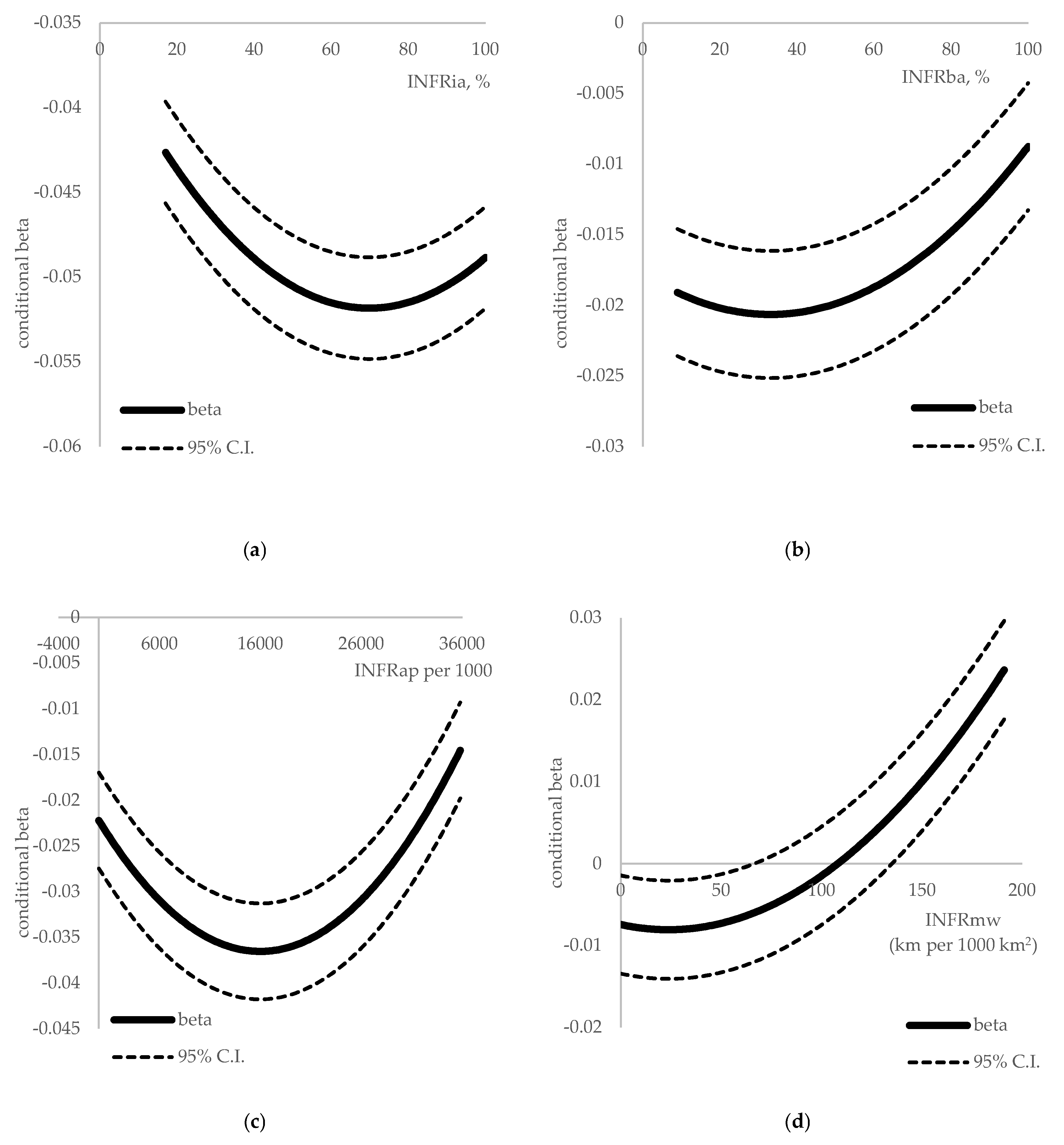
Estimation results on the impact of infrastructure development on convergence using the fixed effects are presented in

Table 3. Fixed effects estimates of Equation (2). Dependent variable—5-year forward-looking average growth rate.

Full Name of the Regressor	Abbreviation	Parameter	Internet Access	Broadband Access	Air Infrastructure	Road Infrastructure	Railway Infrastructure
Initial per capita GDP	ln(Y)	β	–0.03579 ***	–0.01772 ***	–0.02220 ***	–0.007427 ***	–0.01099 ***
			(0.006066)	(0.004230)	(0.002028)	(0.001786)	(0.002110)
Infrastructure	INFR	γ1	0.003417 ***	0.002026 ***	0.0000187 ***	0.0007632 ***	0.0005623 ***
			(0.0001742)	(0.0001386)	(0.0000056)	(0.0002547)	(0.0002142)
	INFR2	γ2	–0.0000277 ***	–0.0000316 **	–5.714 × 10−10 ***	–0.0000129 ***	–0.0000003 **
			(0.0000015)	(0.0000138)	(3.559 × 10−11)	(0.0000035)	(0.0000001)
Interaction between initial per capita GDP and infrastructure	ln(Y) × INFR	δ1	–0.0004593 **	–0.0001762 ***	–0.0000018 ***	–0.0000536 ***	–0.0000407 *
			(0.0001813)	(0.0000425)	(0.0000005)	(0.0000134)	(0.0000216)
	ln(Y) × INFR2	δ2	0.0000033 **	0.0000027 *	5.611 × 10−11 ***	0.0000011 ***	1.444 × 10−8 **
			(0.0000015)	(0.0000014)	(1.516 × 10−11)	(0.0000005)	(6.056 × 10−9)
Capital investment	k	c1	0.0000015 ***	0.0000019 ***	0.00000141 ***	0.0000030 ***	0.0000022 ***
			(0.0000003)	(0.0000003)	(0.0000003)	(0.0000003)	(0.0000003)
	k2	c2	–3.979 × 10−11 ***	–4.858 × 10−11 ***	–3.531 × 10−11 ***	–5.930 × 10−11 ***	–5.040 × 10−11 ***
			(6.903 × 10−12)	(6.810 × 10−12)	(6.223 × 10−12)	(6.178 × 10−12)	(5.634 × 10−12)
Investment in R&D	r&d	c3	0.001810 ***	0.002268 ***	0.002886 ***	0.003128 ***	0.001454 **
			(0.0005656)	(0.0005974)	(0.0005809)	(0.0004626)	(0.0006528)
Population density	pd	c4	0.0002385	0.0003024	0.002518 ***	0.002222 ***	0.001623 ***
			(0.0004083)	(0.0004388)	(0.0004002)	(0.0004725)	(0.0005275)
Human capital	hc	c5	0.0000971	0.0000826	0.0002051 ***	0.0003477 ***	0.0005330 ***
			(0.0000498)	(0.0000538	(0.0000520)	(0.0000486)	(0.0000540)
Labor force growth	Δln(lf)	c6	0.06593	0.09202 *	0.01617	–0.01694	–0.04087
			(0.04710)	(0.04989)	(0.03759)	(0.03133)	(0.03174)
Quality of the governance	QoG	c7	0.001206 *	0.001486 **	0.004463 ***	0.001975 ***	0.001217 **
			(0.0006404)	(0.0007009)	(0.0005809)	(0.0005578)	(0.0006046)
Weight	W	c8	0.011919 ***	0.00389 *	0.002706	0.010028 ***	0.014023 ***
			(0.001847)	(0.002003)	(0.002152)	(0.002067)	(0.001951)
Intercept	α		0.3067 ***	0.1805 ***	0.2322 ***	0.1068 ***	0.1385 ***
			(0.0549)	(0.0389)	(0.0171)	(0.0150)	(0.0183)
Number of observations			878	870	1186	1646	1527
Number of regions			125	125	124	139	142
The average number of observations per region			7.0	7.0	9.6	11.8	10.8
Within R2			0.7009	0.6769	0.5859	0.6226	0.6581
Test for differing group intercepts (1) [p-value]			[<0.001]	[<0.001]	[<0.001]	[<0.001]	[<0.001]
Breusch-Pegan (2) [p-value]			[<0.001]	[<0.001]	[<0.001]	[<0.001]	[<0.001]
Hausman test (3) [p-value]			[<0.001]	[<0.001]	[<0.001]	[<0.001]	[<0.001]
Wooldridge test (4) [p-value]			[<0.001]	[<0.001]	[<0.001]	[<0.001]	[<0.001]
Wald test for heteroscedasticity (5) [p-value]			[<0.001]	[<0.001]	[<0.001]	[<0.001]	[<0.001]
Pesaran CD test (6) [p-value]			[0.1203]	[0.1470]	[0.1932]	[0.1106]	[0.0700]
Wald joint test on time dummies (7) [p-value]			[<0.001]	[<0.001]	[<0.001]	[<0.001]	[<0.001]

Note: All estimations include time dummies since null on joint insignificance of time dummies was rejected. Since the presence of heteroscedasticity and serial correlation in the error term was detected, heteroscedasticity and serial correlation robust standard errors are presented in parentheses. *, **, *** indicate significance at the 10, 5 and 1 per cent levels, respectively. ⁽¹⁾ A low p-value counts against the null hypothesis that the pooled OLS model is adequate in favor of the fixed effects alternative. ⁽²⁾ A low p-value counts against the null hypothesis that the pooled OLS model is adequate in favor of the random effects alternative. ⁽³⁾ A low p-value counts against the null hypothesis that the random-effects model is consistent in favor of the fixed-effects model. ⁽⁴⁾ A low p-value counts against the null hypothesis: no first-order serial correlation in error terms. ⁽⁵⁾ A low p-value counts against the null hypothesis: heteroscedasticity is not present. ⁽⁶⁾ A low p-value counts against the null hypothesis: cross-sectional independence. ⁽⁷⁾ A low p-value counts against the null hypothesis: no time effects.

and graphical representation of this relationship is in Figure 1.

Estimates show that the relationship between infrastructure development and regional convergence is non-linear and that extensive development of infrastructure in some regions, probably at the expense of others, can slow down the convergence. We estimate that convergence is fastest if internet access is at approximately 70%, broadband at 33%, air passengers per one thousand inhabitants is approximately 16,000, and the length of motorways per 1000 km² is 25. Above that level, convergence is still present but at a slower rate, except for the motorway infrastructure. Highly developed motorway infrastructure (the level above 110 km per 1000 km²) in a few regions, with others lagging behind, could even trigger a divergence. Considering the railway infrastructure, its development is also nonlinearly linked to convergence with a diminishing marginal impact, but we do not see a tipping point over the range of the observed values.

For the robustness check, we re-estimated Equation (2) using a 3-year forward-looking average growth rate as the dependent variable. Estimates are presented in Appendix A (

Table A1. Fixed effects estimates of Equation (2). Dependent variable—3-year forward-looking average growth rate.

Full Name of the Regressor	Abbreviation	Parameter	Internet Access	Broadband Access	Air Infrastructure	Road Infrastructure	Railway Infrastructure
Initial per capita GDP	ln(Y)	β	–0.03473 ***	–0.01331 **	–0.02018 ***	–0.005149 **	–0.008521 ***
			(0.007768)	(0.005373)	(0.002496)	(0.002220)	(0.002661)
Infrastructure	INFR	γ1	0.004046 ***	0.00282 **	0.000023 ***	0.001177 ***	0.000397 **
			(0.001231)	(0.000761)	(0.0000069)	(0.000141)	(0.0001702)
	INFR2	γ2	–0.000037 **	–0.000037 **	–9.230 × 10−10 **	–0.000038 **	–6.694 × 10−8 **
			(0.000016)	(0.000018)	(4.381 × 10−10)	(0.000012)	(3.851 × 10−7)
Interaction between initial per capita GDP and infrastructure	ln(Y) × INFR	δ1	–0.0005158 **	–0.001567 ***	–0.000002 ***	–0.000089 **	–0.000033 ***
			(0.0002321)	(0.0005810)	(6.789 × 10−7)	(0.000039)	(0.000017)
	ln(Y) × INFR2	δ2	4.072 × 10−6 **	3.023 × 10−6 **	9.091 × 10−6 **	2.612 × 10−6 **	3.333 × 10−11 **
			(1.952 × 10−6)	(1.449 × 10−6)	(4.328 × 10−11)	(1.105 × 10−6)	(1.638 × 10−8)
Capital investment	k	c1	1.863 × 10−6 ***	2.325 × 10−6 ***	1.937 × 10−6 ***	3.388 × 10−6 ***	2.754 × 10−6 ***
			(4.255 × 10−7)	(4.348 × 10−7)	(3.902 × 10−7)	(3.717 × 10−7)	(3.756 × 10−7)
	k2	c2	–4.525 × 10−11 ***	–5.489 × 10−11 ***	–4.209 × 10−11 ***	–6.424 × 10−11 ***	–5.658 × 10−11 ***
			(8.840 × 10−12)	(8.650 × 10−12)	(7.660 × 10−12)	(7.683 × 10−12)	(7.105 × 10−12)
Investment in R&D	r&d	c3	0.001430 **	0.001888 **	0.002765 ***	0.002871 ***	0.003167 ***
			(0.000724)	(0.000759)	(0.000715)	(0.000575)	(0.000823)
Population density	pd	c4	0.000184	0.000315	0.002091 ***	0.002110 ***	0.002332 ***
			(0.000523)	(0.000558)	(0.000493)	(0.000588)	(0.000665)
Human capital	hc	c5	0.000094	0.000094	0.000245 ***	0.000398 ***	0.000597 ***
			(0.000064)	(0.000068)	(0.000064)	(0.000060)	(0.000068)
Labor force growth	Δln(lf)	c6	0.1053 *	0.1385 *	0.07925 *	0.05019	0.01582
			(0.06032)	(0.08337)	(0.04627)	(0.03896)	(0.04003)
Quality of the governance	QoG	c7	0.001635 **	0.002258 **	0.003825 ***	0.001287 *	0.001414 **
			(0.000820)	(0.000890)	(0.000715)	(0.000693)	(0.000703)
Weight	W	c8	0.006793 ***	0.002309 *	0.002529 *	0.008656 ***	0.004144 ***
			(0.001099)	(0.001327)	(0.001444)	(0.001205)	(0.001154)
Intercept	α		0.3195 ***	0.1674 ***	0.2182 ***	0.08742 ***	0.1211 ***
			(0.07032)	(0.04936)	(0.02104)	(0.01868)	(0.02310)
Number of observations			878	870	1186	1646	1527
Number of regions			125	125	124	139	142
The average number of observations per region			7.0	7.0	9.6	11.8	10.8
Within R2			0.6400	0.6170	0.5356	0.5794	0.5994
Test for differing group intercepts (1) [p-value]			[<0.001]	[<0.001]	[<0.001]	[<0.001]	[<0.001]
Breusch–Pegan (2) [p-value]			[<0.001]	[<0.001]	[<0.001]	[<0.001]	[<0.001]
Hausman test (3) [p-value]			[<0.001]	[<0.001]	[<0.001]	[<0.001]	[<0.001]
Wooldridge test (4) [p-value]			[<0.001]	[<0.001]	[<0.001]	[<0.001]	[<0.001]
Wald test for heteroscedasticity (5) [p-value]			[<0.001]	[<0.001]	[<0.001]	[<0.001]	[<0.001]
Pesaran CD test (6) [p-value]			[0.1300]	[0.0790]	[0.0946]	[0.1567]	[0.1070]
Wald joint test on time dummies (7) [p-value]			[<0.001]	[<0.001]	[<0.001]	[<0.001]	[<0.001]

Note: All estimations include time dummies since null on joint insignificance of time dummies was rejected. Since the presence of heteroscedasticity and serial correlation in the error term was detected, heteroscedasticity and serial correlation robust standard errors are presented in parentheses. *, **, *** indicate significance at the 10, 5 and 1 per cent levels, respectively. ⁽¹⁾ A low p-value counts against the null hypothesis that the pooled OLS model is adequate in favor of the fixed effects alternative. ⁽²⁾ A low p-value counts against the null hypothesis that the pooled OLS model is adequate in favor of the random effects alternative. ⁽³⁾ A low p-value counts against the null hypothesis that the random-effects model is consistent in favor of the fixed-effects model. ⁽⁴⁾ A low p-value counts against the null hypothesis: no first-order serial correlation in error terms. ⁽⁵⁾ A low p-value counts against the null hypothesis: heteroscedasticity is not present. ⁽⁶⁾ A low p-value counts against the null hypothesis: cross-sectional independence. ⁽⁷⁾ A low p-value counts against the null hypothesis: no time effects.

). Additionally, using the same 5-year forward-looking average growth rate as the dependent variable, we re-estimated Equation (2) applying system GMM. Estimates are presented in Appendix A (

Table A2. System GMM estimates of Equation (2). Dependent variable—5-year forward-looking average growth rate.

Full Name of the Regressor	Abbreviation	Parameter	Internet Access	Broadband Access	Air Infrastructure	Road Infrastructure	Railway Infrastructure
Initial per capita GDP	ln(Y)	β	–0.034329 ***	–0.018307 ***	–0.020844 ***	–0.006809 ***	–0.011820 ***
			(0.005464)	(0.004174)	(0.001952)	(0.001737)	(0.001962)
Infrastructure	INFR	γ1	0.003325 ***	0.001971 ***	0.000017 ***	0.000733 ***	0.000583 **
			(0.000187)	(0.000139)	(0.000005)	(0.000232)	(0.000235)
	INFR2	γ2	–0.000029 ***	–0.000029 **	–5.758 × 10−10 ***	–0.000013 ***	–2.795817 × 10−7 ***
			(0.000002)	(0.000014)	(3.647 × 10−11)	(0.000004)	(9.696 × 10−8)
Interaction between initial per capita GDP and infrastructure	ln(Y) × INFR	δ1	–0.000488 ***	–0.000168 ***	–1.918 × 10−6 ***	–0.000050 ***	–0.000042 **
			(0.000164)	(0.000045)	(5.21393)	(0.000013)	(0.000020)
	ln(Y) × INFR2	δ2	3.358 × 10−6 **	2.602 × 10−6 **	5.598 × 10−11 ***	1.082 × 10−6 **	1.441 × 10−8 **
			(1.415 × 10−6)	(1.289 × 10−6)	(1.499 × 10−11)	(4.839 × 10−7)	(6.357 × 10−9)
Capital investment	k	c1	1.588 × 10−6 ***	1.805 × 10−6 ***	1.351 × 10−6 ***	3.164 × 10−6 ***	2.262 × 10−6 ***
			(3.064 × 10−7)	(2.956 × 10−7)	(3.083 × 10−7)	(2.819 × 10−7)	(2.786 × 10−7)
	k2	c2	–3.825 × 10−11 ***	–5.172 × 10−11 ***	–3.196 × 10−11 ***	–5.846 × 10−11 ***	–4.801 × 10−11 ***
			(6.232 × 10−12)	(6.933 × 10−12)	(6.027 × 10−12)	(6.013 × 10−12)	(5.802 × 10−12)
Investment in R&D	r&d	c3	0.001706 ***	0.002155 ***	0.002899 ***	0.003253 ***	0.001465 ***
			(0.000547)	(0.000625)	(0.000627)	(0.000419)	(0.000605)
Population density	pd	c4	0.000238	0.000309	0.002746 ***	0.002013 ***	0.001578 ***
			(0.000446)	(0.000448)	(0.000391)	(0.000511)	(0.000477)
Human capital	hc	c5	0.000098 **	0.000085	0.000217 ***	0.000358 ***	0.000502 ***
			(0.000049)	(0.000059)	(0.000054)	(0.000046)	(0.000055)
Labor force growth	Δln(lf)	c6	0.060923	0.098666 *	0.016697	−0.018018	−0.038230
			(0.042506)	(0.051980)	(0.039669)	(0.032197)	(0.028998)
Quality of the governance	QoG	c7	0.001227 **	0.001501 **	0.004530 ***	0.001943 ***	0.001252 **
			(0.000611)	(0.000661)	(0.000633)	(0.000518)	(0.000550)
Weight	W	c8	0.011838 ***	0.003601 *	0.002976	0.011007 ***	0.013757 ***
			(0.001965)	(0.001840)	(0.002100)	(0.001979)	(0.001919)
Intercept	α		0.326625 ***	0.192803 ***	0.233057 ***	0.097840 ***	0.131390 ***
			(0.059174)	(0.040624)	(0.016901)	(0.014485)	(0.017133)
Y(−1)			0.62502 ***	0.6069 ***	0.64481 ***	0.62228 ***	0.6749 ***
			(0.0607543)	(0.06731933)	(0.06076723)	(0.06407881)	(0.06535224)
Number of observations			878	870	1186	1646	1527
Number of regions			125	125	124	139	142
The average number of observations per region			7.0	7.0	9.6	11.8	10.8
Number of Instruments			113	120	119	127	124
Sargan test (1) [p-value]			[0.202]	[0.228]	[0.234]	[0.254]	[0.222]
Hansen test (1) [p-value]			[0.206]	[0.210]	[0.228]	[0.255]	[0.216]
AR(2) test (2) [p-value]			[0.130]	[0.161]	[0.177]	[0.106]	[0.171]

Note: All estimations are 2-steps system GMM including equations in levels. Once the 1-step estimator is computed, the sample covariance matrix of the estimated residuals is used to obtain 2-step estimates, which are not only consistent but also asymptotically efficient. All estimations include time dummies. Robust (Windmeijer-corrected) standard errors are presented in parentheses. To take into account the concern about the downward-biased tendency of standard errors estimated by the system GMM approach for small samples, we used finite-sample Windmeijer corrections to the asymptotic covariance matrix of the parameters, which are nowadays almost universally used. *, **, *** indicate significance at the 10, 5 and 1 per cent levels, respectively. ⁽¹⁾ A low p-value counts against the null hypothesis of no model misspecification. ⁽²⁾ A low p-value counts against the null hypothesis of no second-order autocorrelation.

). Results are consistent with our general estimations showing a non-linear relationship between infrastructure development and growth and a negative effect of infrastructure concentration on regional convergence.

4. Discussion and Policy Implications

In our study of the impact of infrastructure development on convergence, we found some expected results, but some were surprising. As expected, the estimations revealed that conditional beta convergence between EU NUTS 2 regions is present. It is in line with Bisciari, Essers & Vincent [31], Butkus, Mačiulytė-Šniukienė & Matuzevičiūtė [32], Cartone, Postiglione, & Hewings [33] findings. However, regional economic disparities are still substantial [11], and the rate of convergence is slow. Therefore, policymakers need to make decisions that would promote convergence. Our analysis shows that economic growth is positively related to capital investment, investment in R&D, human capital, the quality of governance, and agglomeration. Therefore, to encourage convergence, it is expedient to increase capital investment, support the creation and spread of innovation, implement human capital development programs, and ensure government quality in economically weaker regions whose GDP per capita is below the EU average. According to Collin & Weil’s [34] findings, human capital investments have a more significant effect than physical capital investments. Achieving inclusive, smart, and sustainable growth requires knowledge and skills [35]. Sharma, Sousa and Woodward [36] describe innovation as a key driver of economic growth and competitiveness. However, one of the factors of innovation development is human capital [37]. Diebolt & Hippe [37] carried out the research using a large data set from the 19th and 20th centuries and revealed that human capital is a vital factor of innovation and the economic status of European regions. Thus, the mentioned factors are related to each other. However, the determination of investment priorities and the efficiency of their use depend on the quality of the government. Thus, the institutional environment influences physical and human capital [38], development and innovations [39].

The result of the study that agglomeration is one of the factors positively influencing economic growth is also not surprising. According to Iammarino et al. [40], agglomeration generates positive economic externalities. Agglomeration reduces barriers to knowledge transfers and simultaneously promotes the development of innovations. However, whether this is a sufficient reason to promote agglomeration is debatable. Although investments in big cities are more effective and positively affect the country-wide economy [40], they also promote regional socio-economic inequality [41]. To make recommendations on the promotion (or limitation) of agglomeration, a separate study, which would allow for weighing its benefits and harm, would be required. According to Capello & Cerisola [42], EU Cohesion funds should be directed to all areas (strong and weak) according to specific needs and potential.

Based on capital investment theory, we expected that the relationship between infrastructure (in this case, transport and ICT) is non-linear. Research has confirmed this insight. We also estimated a threshold level when further infrastructure development has no positive marginal effect on growth. However, what was unexpected was that although investments in infrastructure in EU countries are very intensive, the development of infrastructure in almost all NUTS 2 regions does not reach the estimated threshold level.

On the one hand, this means that seeking to encourage the growth of less developed EU regions is appropriate to develop the transport and ICT infrastructure even more intensively and increase the volume of investments. On the other hand, it could be that regions’ governments do not ensure the potential effectiveness of investments. In this case, more efficient allocation and usage of infrastructure investments would ensure greater development without increasing infrastructure investments. Especially since studies show that the effectiveness of investments depends on government quality, which varies in EU countries and regions, and is very low in some. Yet, additional research is needed to confirm this. It could be a direction for further study. However, there is a problem of a lack of data. Databases do not provide data on the volume of investment in infrastructure by type of infrastructure, especially at the regional level.

Thus, policymakers should first ensure the accumulation of data on investments (private, public, support) at the national and regional level and their public availability. This issue was also mentioned by Timilsina and Hochman [20]. Nevertheless, research on infrastructure development using physical volume indicators makes it possible to form certain policy implications. Before that, it is appropriate to analyze what policy implications are provided by authors in previous papers (see

Table 4. Policy implications provided in previous papers investigating transport and ICT infrastructure development outcomes.

Source	Sample	Period	Policy Implications
Transport Infrastructure
Crescenzi & Rodríguez-Pose [21]	EU–15, NUTS1 & NUTS2	1990–2004	To strengthen the assessment of infrastructure projects, considering benefits and costs and comparing them with alternative uses of the same resources.
Farhadi [22]	18 OECD countries	1870–2009	To invest in projects with a positive real rate of returns.
Cigu et al. [16]	EU–28 countries	2000–2014	To consolidate a viable strategy that makes public policy outcomes more responsible. Policymakers must strive to make public institutions work efficiently by consolidating opportunities and Musgravian indicators.
Lenz et al. [15]	CEE MS	1995–2016	To invest more into railway infrastructure because most investment was directed to developing and modernizing motorways.
Kyriacou et al. [17]	34 countries (24 of them EU MS)	1996–2010	To increase TII efficiency, countries should improve the capacity of the public administration and reduce public sector corruption.
ICT Infrastructure
Pradhan et al. [23]	G-20 countries	2001–2012	To expand and upgrade ICT infrastructure, focusing on the adaptation of the broadband and internet.
Toader et al. [18]	EU-28	2000–2017	To increase investments in ICT and facilitate access to these technologies.
Cioacă et al. [43]	EU-28	2008–2018	To refine digitalization strategy and increase investments to ensure a single digital market that reduces social inequality.
Fernández-Portillo [44]	EU countries that belong OECD	2014–2017	To increase ICT investments, their allocation between projects must be based on cost-benefit analysis.
Maneejuk & Yamaka [45]	5 developed, 5 developing countries	1995–2017	To improve and develop mobile phone infrastructure in both developed and developing countries. To improve ICT industry.
Nair et al. [24]	36 OECD countries	1961–2018	To ensure a holistic co-development policy covering and bridging increase of ICT adaptation, R&D augment and economic growth.

).

Most of the authors [18,21,22,23,24], evaluating transport and ICT infrastructure outcomes provide very general recommendations for policymakers. Some authors [14,31,46,47] did not offer any policy implications focusing more on theoretical and/or methodological insights. Furthermore, they provide results and some insights that can be useful for forming investment allocation policies. Crescenzi & Rodríguez-Pose [21] and Fernández-Portillo [44] concluded that the investment allocation could be based on a project cost-benefit analysis. However, it is not easy to implement this suggestion in practice because the application evaluation period is quite short. Moreover, it would not ensure the direction of investments to the regions where infrastructure development is most needed. Another issue is related to corruption. Projects may not be evaluated objectively in regions with a high level of corruption. It would be more appropriate to determine the optimal infrastructure level and direct investment to regions that have not reached this level.

Our research confirms the non-linear relationship between transport and ICT infrastructure development and regions’ convergence. Estimation revealed the optimal level of infrastructure development which is speeding-up convergence. This optimal level of development has been exceeded in some regions. Regarding the development of motorways, the optimal level was exceeded in 78 EU NUTS 2 regions, the optimal level was reached in 7 regions, and not in 80 regions in 2019 (see Appendix B,

Table A3. EU regions divided into groups according to whether they exceeded or not motorways development threshold level.

No	Region Code	Region	Length of Motorways per 1000 km2	No	Region Code	Region	Length of Motorways per 1000 km2
Threshold Level			25	Threshold Level			25
1	BG31	Severozapaden	1	1	BE10	Région de Bruxelles-Capitale/Brussels Hoofdstedelijk Gewest	70
2	BG33	Severoiztochen	7	2	BE21	Prov. Antwerpen	77
3	BG34	Yugoiztochen	11	3	BE22	Prov. Limburg (BE)	44
4	BG41	Yugozapaden	13	4	BE23	Prov. Oost-Vlaanderen	66
5	BG42	Yuzhen tsentralen	9	5	BE24	Prov. Vlaams-Brabant	83
6	CZ03	Jihozápad	10	6	BE25	Prov. West-Vlaanderen	60
7	CZ04	Severozápad	15	7	BE31	Prov. Brabant wallon	57
8	CZ05	Severovýchod	3	8	BE32	Prov. Hainaut	75
9	CZ06	Jihovýchod	18	9	BE33	Prov. Liège	69
10	CZ07	Strední Morava	19	10	BE34	Prov. Luxembourg (BE)	35
11	CZ08	Moravskoslezsko	18	11	BE35	Prov. Namur	28
12	DK04	Midtjylland	25	12	CZ01	Praha	90
13	DK05	Nordjylland	24	13	CZ02	Strední Cechy	32
14	DE80	Mecklenburg- Vorpommern	25	14	DK01	Hovedstaden	65
15	DEE0	Sachsen-Anhalt	24	15	DK02	Sjælland	39
16	EE00	Eesti	4	16	DK03	Syddanmark	31
17	IE04	Northern and Western	3	17	DE30	Berlin	86
18	IE05	Southern	17	18	DE40	Brandenburg	27
19	IE06	Eastern and Midland	24	19	DE50	Bremen	191
20	ES41	Castilla y León	25	20	DE60	Hamburg	101
21	ES42	Castilla-la Mancha	23	21	DEC0	Saarland	93
22	ES43	Extremadura	17	22	DEF0	Schleswig-Holstein	34
23	ES53	Illes Balears	19	23	DEG0	Thüringen	32
24	FRB0	Centre—Val de Loire	25	24	ES11	Galicia	38
25	FRC1	Bourgogne	22	25	ES12	Principado de Asturias	43
26	FRC2	Franche-Comté	13	26	ES13	Cantabria	48
27	FRD1	Basse-Normandie	16	27	ES21	País Vasco	69
28	FRF2	Champagne-Ardenne	21	28	ES22	Comunidad Foral de Navarra	37
29	FRF3	Lorraine	20	29	ES23	La Rioja	36
30	FRG0	Pays-de-la-Loire	23	30	ES30	Comunidad de Madrid	95
31	FRH0	Bretagne	2	31	ES51	Cataluña	46
32	FRI1	Aquitaine	21	32	ES52	Comunitat Valenciana	51
33	FRI2	Limousin	16	33	ES61	Andalucía	30
34	FRI3	Poitou-Charentes	12	34	ES62	Región de Murcia	53
35	FRJ1	Languedoc-Roussillon	22	35	ES70	Canarias	37
36	FRJ2	Midi-Pyrénées	14	36	FR10	Île de France	52
37	FRK1	Auvergne	15	37	FRD2	Haute-Normandie	36
38	FRL0	Provence-Alpes-Côte d’Azur	24	38	FRE1	Nord-Pas-de-Calais	50
39	ITH5	Emilia-Romagna	25	39	FRE2	Picardie	29
40	ITI1	Toscana	20	40	FRF1	Alsace	36
41	ITI2	Umbria	7	41	FRK2	Rhône-Alpes	29
42	ITI3	Marche	18	42	HR03	Jadranska Hrvatska	26
43	ITF2	Molise	8	43	ITC1	Piemonte	33
44	ITF4	Puglia	16	44	ITC2	Valle d’Aosta/Vallée d’Aoste	35
45	ITF5	Basilicata	3	45	ITC3	Liguria	69
46	ITF6	Calabria	19	46	ITC4	Lombardia	30
47	ITG2	Sardegna	18	47	ITH1	Provincia Autonoma di Bolzano/Bozen	29
48	LT01	Sostines regionas	10	48	ITH3	Veneto	32
49	LT02	Vidurio ir vakaru Lietuvos regionas	4	49	ITH4	Friuli-Venezia Giulia	27
50	HU21	Közép-Dunántúl	24	50	ITI4	Lazio	29
51	HU22	Nyugat-Dunántúl	20	51	ITF1	Abruzzo	33
52	HU23	Dél-Dunántúl	21	52	ITF3	Campania	32
53	HU31	Észak-Magyarország	13	53	ITG1	Sicilia	27
54	HU32	Észak-Alföld	13	54	CY00	Kypros	28
55	HU33	Dél-Alföld	12	55	LU00	Luxembourg	64
56	AT11	Burgenland (AT)	20	56	HU11	Budapest	120
57	AT12	Niederösterreich	20	57	HU12	Pest	39
58	AT21	Kärnten	25	58	NL11	Groningen	36
59	AT22	Steiermark	19	59	NL12	Friesland (NL)	36
60	AT31	Oberösterreich	25	60	NL13	Drenthe	55
61	AT32	Salzburg	20	61	NL21	Overijssel	52
62	AT33	Tirol	15	62	NL22	Gelderland	79
63	AT34	Vorarlberg	24	63	NL23	Flevoland	43
64	PL21	Malopolskie	10	64	NL31	Utrecht	128
65	PL22	Slaskie	17	65	NL32	Noord-Holland	73
66	PL41	Wielkopolskie	7	66	NL33	Zuid-Holland	105
67	PL42	Zachodniopomorskie	1	67	NL34	Zeeland	30
68	PL43	Lubuskie	6	68	NL41	Noord-Brabant	99
69	PL51	Dolnoslaskie	11	69	NL42	Limburg (NL)	96
70	PL52	Opolskie	9	70	AT13	Wien	104
71	PL63	Pomorskie	4	71	RO32	Bucuresti—Ilfov	46
72	PL71	Lódzkie	12	72	SI03	Vzhodna Slovenija	26
73	PL82	Podkarpackie	9	73	SI04	Zahodna Slovenija	38
74	RO11	Nord-Vest	2	74	SK01	Bratislavský kraj	54
75	RO12	Centru	4	75	FI1B	Helsinki-Uusimaa	34
76	RO22	Sud-Est	2	76	SE11	Stockholm	48
77	RO31	Sud—Muntenia	7	77	SE12	Östra Mellansverige	47
78	RO42	Vest	8	78	SE22	Sydsverige	26
79	SK02	Západné Slovensko	10
80	SK03	Stredné Slovensko	6
81	SK04	Východné Slovensko	8
82	FI19	Länsi-Suomi	2
83	FI1C	Etelä-Suomi	10
84	FI1D	Pohjois- ja Itä-Suomi	1
85	SE21	Småland med öarna	6
86	SE31	Norra Mellansverige	1
87	SE32	Mellersta Norrland	22

). It should be noted that there is no data on regional motorways development in Greece, Latvia, Malta, and Portugal. In addition, there is a lack of data for some regions in other countries. The study revealed that motorways development is uneven in all countries. There worst situation is in Romania, where motorways development reached an optimal level only in one region. Based on research results, the intensity of investments in motorways development should be increased for the regions of Romania (except for Bucuresti—Ilfov, RO32 region), Bulgaria, Chechia (except for the Prague, CZ01, and Strední Cechy, CZ020 regions), Estonia, Lithuania and Poland and some regions of other countries.

Regarding ICT development, estimations reveal that their positive impact on convergence is slowing down when households with access to the internet at home exceed 70% and households with broadband access exceed 33%. According to Eurostat data, this threshold level exceeded all EU MS NUTS 2 regions, except Severoiztochen (BG33) region, where households’ access to the internet was 66%. It can be argued that internet and broadband development should not be supported in the future. Maciulyte-Sniukiene & Butkus [19] concluded that the development of mobile networks should be supported at the country level. However, it is not possible to determine the impact of mobile networks on convergence at the regional level due to the lack of data.

Our results are not in line with Pradhan et al.’s [23] and Toader et al.’s [18] conclusion that investments must be directed to expanding ICT infrastructure, focussing on broadband and the internet. As this study has shown, internet and broadband networks are sufficiently expanded in all EU countries and regions. Therefore, the focus should be placed on the development of mobile networks. Nowadays, mobile connectivity plays an essential role in the digital connection of people and businesses to the internet, the cloud, and each other [48]. Mobile technologies and systems support the effective delivery of public services and learning opportunities for societies [19].

The number of air passengers per one thousand inhabitants exceeded the established threshold level, after which air infrastructures’ positive impact on convergences slowdowns was exceeded just in 28 NUTS 2 regions (see Appendix C,

Table A4. EU NUTS 2 regions where air passengers per one thousand inhabitants exceeded 16,000 in 2019.

No	Region Code	Region	Air Passengers per One Thousand Inhabitants	No	Region Code	Region	Air Passengers per One Thousand Inhabitants
Threshold Level			Approx. 16,000	Threshold Level			Approx. 16,000
1	CZ01	Praha	17,839	15	ES70	Canarias	40,035
2	DK01	Hovedstaden	30,135	16	FR10	Île de France	107,991
3	DE21	Oberbayern	47,892	17	FRL0	Provence-Alpes-Côte d’Azur	25,090
4	DE30	Berlin	24,223	18	ITC4	Lombardia	49,096
5	DE60	Hamburg	17,274	19	ITH3	Veneto	18,404
6	DE71	Darmstadt	70,436	20	ITI4	Lazio	49,250
7	DEA1	Düsseldorf	26,707	21	ITG1	Sicilia	18,182
8	IE06	Eastern and Midland	32,653	22	HU11	Budapest	16,100
9	EL30	Attiki	25,578	23	NL32	Noord-Holland	71,690
10	ES30	Comunidad de Madrid	59,747	24	AT12	Niederösterreich	31,635
11	ES51	Cataluña	54,693	25	PL91	Warszawski stoleczny	21,972
12	ES52	Comunitat Valenciana	23,401	26	PT17	Área Metropolitana de Lisboa	31,204
13	ES53	Illes Balears	40,285	27	FI1B	Helsinki-Uusimaa	22,049
14	ES61	Andalucía	30,414	28	SE11	Stockholm	27,993

). Yet, to provide clear recommendations for policymakers, the development of air transport for freight, not only for passengers, should be evaluated. It requires additional data at the NUTS 2 level. According to European Commission [49], the most significant focus should be on increasing accessibility of airports using high-speed trains and other conventional and innovative modes of transport and reducing air transport and airport carbon footprint.

According to Nair et al. [24], countries’ and regions’ development policies have to be holistic and cover different economic growth factors. Our research results support the insights of Nair et al. [24]. According to our research, regions’ development policies have to encourage the growth of human capital, innovations, and some critical infrastructure and ensure a favorable environment; the essential component is the quality of institutions.

Specific suggestions for investment allocation policy that emerged from this study results are presented in the conclusions section.

5. Conclusions

Analysis of previous studies on core infrastructure outcomes revealed the need for more research on convergence outcomes at the regional level since the effects on economic growth are the most studied. It was also found that the linear effects between infrastructure development and its return variables (usually GDP per capita) are studied, and non-linear effects remain unexplored. Moreover, based on research results, most of the authors provide very general policy implications.

We developed an econometric model to fill those gaps. Results presented in the previous chapter allow us to present policy implications that have not yet been presented in previous studies.

Specific recommendations for structural fund support and investment policymakers:

-

Distribution of investment and support according to smaller regional units, i.e., NUTS 2 level. It would enable a more even development of infrastructure in regions. It might be appropriate to distribute the funds according to even smaller regions (NUTS 3 level). Still, due to the lack of data, conducting a study at this level is impossible;

-

Obligate countries’ governments to collect and publicly (in Eurostat) announce information on national and regional investments, broken down by their types. Provide a support budget (investment volume) for each type of critical infrastructure. It would allow for determining which investments in infrastructure development generate the most significant positive benefits;

-

Establish a tipping point, after which investments no longer generate positive economic outcomes for each type of infrastructure and control that assets do not exceed this threshold. When distributing national investments and support between regions, assess the distance to this threshold, and promote infrastructure development more intensively in regions with more significant gaps;

-

Establish the optimal level of infrastructure development that ensure convergence of regions for each type of infrastructure. It would allow EU investments to be directed to those regions that have not reached this level. Countries’ governments may develop infrastructure in regions where optimal development is achieved or exceeded. However, it should be financed from the national and regional budgets without support.

The study contributes to science and practice in a few ways: (i) The specification that enables estimating the non-linear impact of transport and ICT infrastructure development on convergence was developed. The proposed specification can be used to investigate the non-linear relationship between other types of infrastructure and countries or regions’ convergence, as well as in different regional disaggregation. (ii) It has been proven that the relationship between transport and ICT infrastructure and economic growth and convergence can be non-linear, i.e., the diminishing return effect occurs; (iii) A tipping point of infrastructure development has been determined, after which further development no longer generates positive returns.

Unfortunately, the study has limitations. First, the study only investigates the impact of some types of critical infrastructure on economic growth and convergence due to a lack of regional level data. The study does not include energy, water and sanitation infrastructure. Another limitation is that investigations do not take into account structural breaks. This could be one of the directions for further research. Although the volumes of Structural Funds support are not separately broken down by all types of infrastructure, it would be possible to study the outcomes of Structural Funds support by investment groups presented in the reports (Network Infrastructures in Transport and Energy; Information & Communication Technologies) [50]. In this case, exploring the infrastructure investments’ outcomes in separate programming periods would be possible. In addition, it would make sense to investigate the differences in the returns on infrastructure development between EU member states in Western Europe and Central and Eastern Europe. It is also appropriate to study the impact of infrastructure development on social indicators (e.g., quality of life).

References

- Regulation (EU) 2021/1058 of the Eurpean Parlament and of the Council of 24 June 2021 on the European Regional Development Funds and on the Cohesion Fund. Off. J. Eur. Union 2021, L231, 60–93. Available online: https://eur-lex.europa.eu/legal-content/EN/TXT/?uri=CELEX:32021R1058 (accessed on 10 November 2022).
- European Commission. European Regional Development Funds (ERDF). Cohesion Open Data Platform. Available online: https://cohesiondata.ec.europa.eu/funds/erdf/21-27 (accessed on 10 November 2022).
- European Commission. Cohesion funds (CF). Cohesion Open Data Platform. Available online: https://cohesiondata.ec.europa.eu/funds/cf/21-27 (accessed on 10 November 2022).
- Pinho, C.; Varum, C.; Antunes, M. Structural Funds and European Regional Growth: Comparison of Effects among Different Programming Periods. Eur. Plan. Stud. 2015, 23, 1302–1326. [Google Scholar] [CrossRef] [Green Version]
- Becker, S.O.; Egger, P.; von Ehrlich, M. Effects of EU Regional Policy: 1989–2013. Reg. Sci. Urban Econ. 2018, 69, 143–152. [Google Scholar] [CrossRef]
- Cerqua, A.; Pellegrini, G. Are we spending too much to grow? The case of Structural Funds. J. Reg. Sci. 2018, 58, 535–563. [Google Scholar] [CrossRef]
- Crescenzi, R.; Giua, M. One or many Cohesion Policies of the European Union? On the differential economic impact of Cohesion Policy across member states. Reg. Stud. 2020, 54, 10–20. [Google Scholar] [CrossRef] [Green Version]
- López-Bazo, E. The Impact of Cohesion Policy on Regional Differences in Suport for the European Union. J. Common Mark. Stud. 2022, 60, 1219–1236. [Google Scholar] [CrossRef]
- SWECO. Final Report—ERDF and CF Regional Expenditure Contract. 2007.CE.16.0.AT.036. 2008. Available online: https://ec.europa.eu/regional_policy/sources/docgener/evaluation/pdf/expost2006/expenditure_final.pdf (accessed on 15 November 2022).
- Charron, N.; Lapuente, V.; Rothstein, B. (Eds.) Measuring the Quality of Government and Subnational Variation. Report for the European Commission Directorate-General Regional Policy, Directorate Regional Policy; Quality of Quality of Government and Returns of Investment: Cohesion Expenditure in European Regions 1289 Government Institute, Department of Political Science; University of Gothenburg: Gothenburg, Sweden, 2010. Available online: http://ec.europa.eu/regional_policy/sources/docgener/studies/pdf/2010_government_1.pdf (accessed on 15 July 2019).
- Ciffolilli, A.; Condello, S.; Pompili, M.; Roemish, R. Geography of Expenditure. Final Report. Work Package 13. Ex post evaluation of Cohesion Policy programmes 2007–2013, Focusing on the European Regional Development Fund (ERDF) and the Cohesion Fund (CF). 2015. Available online: https://ec.europa.eu/regional_policy/sources/docgener/evaluation/pdf/expost2013/wp13_final_report_en.pdf (accessed on 15 July 2019).
- European Commission. Measuring the Impact of Structural and Cohesion Funds Using Regression Discontinuity Design in EU27 in the Period 1994-2011, Ex Post Evaluation of Cohesion Policy Programmes 2007–2013, Focusing on the European Regional Development Fund (ERDF) and the Cohesion Fund (CF). Final Technical Report, Work Package 14c—Tasks 2 and 3. 2016. Available online: https://ec.europa.eu/regional_policy/en/information/publications/evaluations/2016/measuring-the-impact-of-structural-and-cohesion-funds-using-the-regression-discontinuity-design-final-technical-report-work-package-14c-of-the-ex-post-evaluation-of-the-erdf-and-cf-2007-2013 (accessed on 15 November 2019).
- European Commission. Strategic Report 2019 on the Implementation of the European Structural and Investment Funds. Report from the Commission to the European Parliament, the Council, the European Economic and Social Committee and the Committee of the Regions. Brussels. 2019. Available online: https://eur-lex.europa.eu/resource.html?uri=cellar:84c1014d-20d7-11ea-95ab-01aa75ed71a1.0003.02/DOC_1&format=PDF (accessed on 10 November 2022).
- Meersman, H.; Nazemzadeh, M. The Contribution of Transport Infrastructure to Economic Activity: The case of Belgium. Case Stud. Transp. Policy 2017, 5, 316–324. [Google Scholar] [CrossRef]
- Lenz, N.V.; Skender, H.P.; Adelajda Mirković, P.A. The macroeconomic effects of transport infrastructure on economic growth: The case of Central and Eastern, E.U. member states. Econ. Res. Ekon Istraz. 2018, 31, 1953–1964. [Google Scholar] [CrossRef]
- Cigu, E.; Agheorghiesei, D.T.; Gavriluta (Vatamanu), A.F.; Toader, E. Transport Infrastructure Development, Public Performance and Long-Run Economic Growth: A Case Study for the EU–28 Countries. Sustainability 2019, 11, 67. [Google Scholar] [CrossRef] [Green Version]
- Kyriacou, A.P.; Muinelo-Gallo, L.; Roca-Sagalé, O. The efficiency of transport infrastructure investment and the role of government quality: An empirical analysis. Transp. Policy 2019, 74, 93–102. [Google Scholar] [CrossRef]
- Toader, E.; Firtescu, B.N.; Roman, A.; Anton, S.G. Impact of Information and Communication Technology Infrastructure on Economic Growth: An Empirical Assessment for the EU Countries. Sustainability 2018, 10, 3750. [Google Scholar] [CrossRef]
- Maciulyte-Sniukiene, A.; Butkus, M. Does Infrastructure Development Contribute to EU Countries’ Economic Growth? Sustainability 2022, 14, 5610. [Google Scholar] [CrossRef]
- Timilsina, G.; Hochman, G.; Song, Z. Infrastructure, Economic Growth, and Poverty. A Review; Policy Research Working Paper 9258; World Bank Group: Washington, DC, USA, 2020. [Google Scholar]
- Crescenzi, R.; Rodríguez-Pose, A. Infrastructure and regional growth in the European Union. Pap. Reg. Sci. 2012, 91, 487–513. [Google Scholar] [CrossRef]
- Farhadi, M. Transport infrastructure and long-run economic growth in OECD countries. Transp. Res. Part A 2015, 74, 73–90. [Google Scholar] [CrossRef]
- Pradhan, R.P.; Mallik, G.; Bagchi, T.P. Information communication technology (ICT) infrastructure and economic growth: A causality evinced by cross-country panel data. IIMB Manag. Rev. 2018, 30, 91–103. [Google Scholar] [CrossRef]
- Nair, M.; Pradhan, R.P.; Arvin, M.B. Endogenous dynamics between R&D, ICT and economic growth: Empirical evidence from the OECD countries. Technol. Soc. 2020, 62, 101315. [Google Scholar] [CrossRef]
- Mačiulytė-Šniukienė, A.; Butkus, M.; Davidavičienė, V. Development of the Model to Examine the Impact of Infrastructure on Economic Growth and Convergence. J. Bus. Econ. Manag. 2022, 23, 731–753. [Google Scholar] [CrossRef]
- Barro, R.J.; Sala-i-Martin, X. Convergence. J. Polit. Econom. 1992, 100, 223–251. [Google Scholar] [CrossRef]
- Charron, N.; Dijkstra, L.; Lapuente, V. Regional Governance Matters: Quality of Government within European Union Member States. Reg. Stud. 2014, 48, 68–90. [Google Scholar] [CrossRef]
- Charron, N.; Dijkstra, L.; Lapuente, V. Mapping the regional divide in Europe: A measure for assessing quality of government in 206 European regions. Soc. Indic. Res. 2015, 122, 315–346. [Google Scholar] [CrossRef]
- Charron, N.; Lapuente, V.; Annoni, P. Measuring Quality of Government in EU Regions Across Space and Time. Pap. Reg. Sci. 2019, 98, 1925–1953. [Google Scholar] [CrossRef]
- Charron, N.; Lapuente, V.; Bauhr, M. Sub-national Quality of Government in EU Member States: Presenting the 2021 European Quality of Government Index and Its Relationship with Covid-19 Indicators; Working Paper Series 2021:4; University of Gothenburg: Gothenburg, Sweden, 2021; Available online: https://www.gu.se/sites/default/files/2021-05/2021_4_%20Charron_Lapuente_Bauhr.pdf (accessed on 16 May 2022).
- Bisciari, P.; Essers, D.; Vincent, E. Does the EU convergence machine still work? In National Bank of Belgium Economic Review; National Bank of Belgium: Brussels, Belgium, 2020. [Google Scholar]
- Butkus, M.; Mačiulytė-Šniukienė, A.; Matuzevičiūtė, K. Mediating Effects of Cohesion Policy and Institutional Quality on Convergence between EU Regions: An Examination Based on a Conditional Beta-Convergence Model with a 3-Way Multiplicative Term. Sustainability 2020, 12, 3025. [Google Scholar] [CrossRef] [Green Version]
- Cartone, A.; Postiglione, P.; Hewings, G.J.D. Does economic convergence hold? A spatial quantile analysis on European regions. Econ. Model. 2021, 95, 408–417. [Google Scholar] [CrossRef]
- Collin, M.; Weil, N.D. The Effect of Increasing Human Capital Investment on Economic Growth and Poverty: A Simulation Exercise; Brown University, Department of Economics Working Papers 2020-03; World Bank: Washington, DC, USA, 2020. [Google Scholar]
- Pelinescu, E. The Impact of Human Capital on Economic Growth. Procedia Econ. Financ. 2015, 22, 184–190. [Google Scholar] [CrossRef] [Green Version]
- Sharma, A.; Sousa, C.; Woodward, R. Determinants of innovation outcomes: The role of institutional quality. Technovation 2022, 118, 102562. [Google Scholar] [CrossRef]
- Diebolt, C.; Hippe, R. The Long-Run Impact of Human Capital on Innovation and Economic Growth in the Regions of Europe. In Human Capital and Regional Development in Europe; Frontiers in Economic History; Springer: Cham, Switzerland, 2022. [Google Scholar]
- Adams-Kane, J.; Lim, J.J. Institutional Quality Mediates the Effect of human Capital on Economic Performance. Rev. Dev. Econ. 2016, 20, 426–442. [Google Scholar] [CrossRef]
- Donbesuur, F.; Ampong, G.O.A.; Owusu-Yirenkyi, D.; Chu, D. Innovations and international performance of SMEs: The moderating role of domestic institutional environment. Technol. Forecast Soc. Chang. 2020, 161, 120252. [Google Scholar] [CrossRef]
- Iammarino, S.; Rodriguez-Pose, A.; Storper, M. Porgional inequality in Europe: Evidence, theory and policy implications. J. Econ. Geogr. 2018, 19, 273–298. [Google Scholar] [CrossRef]
- Sanchez Carrera, E.J.; Rombaldoni, R.; Pozzi, R. Socioeconomic inequalities in Europe. Econ. Anal. Policy 2021, 71, 307–320. [Google Scholar] [CrossRef]
- Capello, R.; Cerisola, S. Concentrated versus diffused growth assets: Agglomeration economies and regional cohesion. Growth Chang. 2020, 51, 1440–1453. [Google Scholar] [CrossRef]
- Cioacă, S.-I.; Cristache, S.-E.; Vuţă, M.; Marin, E.; Vuţă, M. Assessing the Impact of ICT Sector on Sustainable Development in the European Union: An Empirical Analysis Using Panel Data. Sustainability 2020, 12, 592. [Google Scholar] [CrossRef]
- Fernández-Potillo, A.; Almodóvar-González, M.; Hernández-Mogollón, R. Impact of ICT development on economic growth. A study of OECD European union countries. Technol. Soc. 2020, 63, 101420. [Google Scholar] [CrossRef]
- Maneejuk, P.; Yamaka, W. An analysis of the impacts of telecommunications technology and innovation on economic growth. Telecomm. Policy 2020, 44, 102038. [Google Scholar] [CrossRef]
- Carruthers, R. Transport Infrastructure. In Economic and Social Development of the Southern and Eastern Mediterranean Countries; Ayadi, R., Dabrowski, M., De Wulf, L., Eds.; Springer: Cham, Switzerland, 2015. [Google Scholar]
- Luz, J.; Reis, J.; Leite, F.A.; Araújo, K.; Moritz, G. Effects of Transport Infrastructure in the Economic Development. In Proceedings of the IFIP International Conference on Advances in Production Management Systems (APMS), Iguassu Falls, Brazil, 3–7 September 2016; Volume 488, pp. 633–640. [Google Scholar]
- Welsh Government. Code of Best Practice on Mobile Phone Network Development for Wales; Welsh Government: Cardiff, UK, 2021.
- European Commission. Study on Urban Mobility Interconnection with Air Transport Infrastructure. In Final Report, 2021; Publications Office of the European Union: Luxembourg, 2021. [Google Scholar]
- European Commission. 2014–2020 ESIF Overview. Available online: https://cohesiondata.ec.europa.eu/overview/14-20 (accessed on 10 November 2022).
Figure 1.
Relationship between different types of infrastructure development and speed of convergence, i.e., the conditional beta coefficient (calculated based on Equation (3)) and its 95% confidence interval (calculated based on Equation (4)). (a) Access to the internet; (b) Access to broadband internet; (c) Airport infrastructure; (d) Motorways infrastructure; (e) Railways infrastructure.