
Traffic Flow Funnels Based on Aircraft Performance for Optimized Departure Procedures


Institute of Logistics and Aviation, Technische Universität Dresden, 01062 Dresden, Germany
*
Authors to whom correspondence should be addressed.
†
These authors contributed equally to this work.
Future Transp. 2022, 2(3), 711-733; https://doi.org/10.3390/futuretransp2030040
Submission received: 29 April 2022
/
Revised: 21 July 2022
/
Accepted: 15 August 2022
/
Published: 22 August 2022
Abstract
:Aircraft departures often follow standardized and restrictive routes intended to guarantee a safe transition to the en-route network. Since the procedures must take the flight performance of many aircraft types into account, they represent a compromise between numerous optima and must be consistent with noise abatement strategies. This paper investigates the concept of departure funnels, in which flights can adopt their optimal profile within a procedural space based on actual flight performance to replace standard routes. For this, an algorithm based on DBSCAN identifies typical traffic flow funnels for a set of radar tracks as reference and individually optimized flight trajectories as preferred funnels. For the latter, an innovative 3D pathfinding grid is developed, which expands dynamically using the specific flight performance of the aircraft type and enables evaluation of operating costs due to wind and fuel consumption. From the clustered traffic flows, a funnel starting at the runway is determined based on the variance of the flight profiles along their mean trajectory. This funnel provides a restricted space for individual trajectory optimization for the day of operation. The procedure is applied using the example of Munich Airport, where the funnel size and the associated fuel-saving potential are determined. The results indicate an average fuel-saving potential of 0.4% with respect to the trip fuel.
1. Introduction
With typically high traffic density and constrained departure and arrival procedures following noise and environmental mitigation, the terminal maneuvering area (TMA) is an airspace volume in which trajectory optimization is a tedious task and, thus, often omitted. Yet, today’s standard procedures often force flights into unfavorable head-wind conditions, and thus away from their optimal trajectory. The potential for optimization in the TMA is, therefore, vast, despite the opposing interests of aviation stakeholders and residents.
As a concept to achieve more efficient trajectories, we propose a method to create traffic flow funnels for departing aircraft. These funnels permit optimization in contained volumes, while completely prohibiting arbitrary flight paths, to maintain predictability for air traffic control (ATC). Unlike the conventional standard instrument departure (SID), a funnel additionally defines a maximum deviation from a mean trajectory laterally and vertically to enable individually optimized climb profiles per flight, e.g., for following the continuous climb operation (CCO) concept of the International Civil Aviation Organization (ICAO) [1]. The funnels are not intended to account for navigation inaccuracies, such as existing tolerance, but provide significantly larger spaces available for optimization. Since the climb profile is impacted by the aircraft-specific flight performance, including varying gross masses and weather, the funneling process requires a smart design methodology to anticipate this variability.
For the trajectory optimization of departures, our established simulation environment TOolchain for Multi-criteria Aircraft Trajectory Optimization (TOMATO) [2] is extended with a dynamic 3D pathfinding grid specifically designed for CCO. For each flight requiring optimization, the 3D grid is created individually using the flight performance of the aircraft type and its actual take-off mass. Since pathfinding algorithms, such as the A*, cannot maintain the individual aircraft state across multiple nodes, the flight performance must be estimated to consider the available climb gradients in the 3D grid. This concept has been examined previously [3], but is extended here with specifically generated tabulated performance using the open aircraft performance model (OpenAP) [4].
For the analysis, two main scenarios are used. As the reference scenario, recorded automatic dependent surveillance-broadcast (ADS-B) track data from Munich Airport (MUC) is used to build the so-called ADS-B funnels that inherit the current procedures and the resulting flight profiles. Then, all departures contained in the ADS-B dataset are optimized freely, i.e., without route restrictions, but towards minimum fuel burn considering individual weather and direct operating costs with TOMATO [2]. These optimized trajectories are then clustered to the optimized funnels using the same funnel algorithm as for ADS-B data. For both the ADS-B and the optimized funnel, the departures are then reoptimized with the constraint to fly inside each funnel on particular days of operation to judge the fuel-saving potential.
The funnel algorithm uses an iterative clustering, consisting of a combined density-based spatial clustering of applications with noise (DBSCAN) [5], a nearest neighbor assignment, and a secondary DBSCAN within the first determined cluster. Based on each of the clusters, a convex hull for each funnel is computed along a mean trajectory with perpendicular rectangles placed at equally spaced intervals. These rectangles form gates consisting of a grid of waypoints for the reoptimization inside the funnels. Figure 1 displays clustered ADS-B departures from the example airport MUC, where each color marks a trajectory cluster used to derive a single funnel.
This section continues with a review of the state of the art regarding trajectory optimization, clustering, and traffic flow funnels. Section 2 starts with an overview of the methodology, before introducing the multi-objective trajectory optimization, including the tabulated performance for the pathfinding; the 3D search grid, and the vertical profile are described. Furthermore, the funnel algorithm and the pathfinding inside those funnels are developed. Section 3 introduces the scenario for the application, which is then used to analyze both the ADS-B funnel and the optimized funnels, as well as the impact on the flight efficiency of the two funnel designs. Section 4 discusses the findings of the study and the applicability of the traffic flow funnels. Conclusions are presented in Section 5 with suggestions for further areas of research.
1.1. Towards 3D Trajectory Optimization
Trajectory optimization for an entire flight is a lively research area, where several approaches have been developed to balance multiple optimization objectives, such as minimum fuel flow, minimum time, or minimum climate impact by reducing contrail formation [6,7]. For operational cost assessment, specific flight performance modeling is crucial for each aircraft-engine combination, including aerodynamic and combustion models. A free and open aircraft performance model is available for commonly used jet-aircraft types with the OpenAP [4,8], which is built on public data sourced from manufacturers, aviation authorities, aircraft surveillance, and flight trials. Due to the mathematical complexity of a flight performance model, the typical approach in trajectory optimization is to separate lateral pathfinding from vertical profile calculation [2,9,10]. Thus, the cost-optimal path is searched only at cruising altitudes, where the aircraft remains the majority of the flight time. In a consecutive step, the flight profile is optimized on the given flight path. This process is often performed iteratively to successively identify the optimal combination of flight path and profile. A number of approaches to 3D pathfinding have been explored, although mostly limited to the cruise phase. Hartjes et al. [7] used optimal control with the Radau pseudospectral method to perform 3D optimization to avoid contrail-inducing regions vertically. Murrieta-Mendoza et al. [11] used a modified Floyd–Warshall algorithm for 3D path optimization in a grid with a 7.5° lateral and a 1000 ft vertical resolution to find optimal cruising conditions, considering the costs required to change altitudes with the EUROCONTROL Base of Aircraft Data (BADA) flight performance model. Focusing on departing flights, the optimization was either performed in relation to an optimal flight profile, which is the CCO [12], or involved optimizing the procedures and the related ATC interaction in the TMA [13]. Another factor in the ground proximity of the TMA is noise, which Tian et al. [14] considered in an arrival fix allocation problem for continuous descent approach (CDO) arrivals.
1.2. Sources of Trajectory Uncertainty during Climb
A central challenge during the climb is the individual nature of the vertical profile, which not only differs among aircraft types but is also affected by various uncertainty sources [15]. Additionally, the characteristics of these uncertainty sources cannot be extracted from ADS-B data and, therefore, require additional estimation or analysis. Zeh et al. [16] analyzed the impact of the take-off mass with an altitude-dependent optimal true air speed (TAS), finding that the resulting vertical trajectory uncertainty was mainly attributed to the mass uncertainty, while an interdependent combination of the mass and the speed intent influenced the along-track uncertainty. Alligier [17] used a neural network trained on ADS-B data to estimate mass and speed intents for climbing aircraft as Gaussian distributions, identifying the transitions between speed intents as an additional factor to the resulting uncertainty besides mass and the speed intent itself. These speed intent transitions, originating in the cross-over from constant CAS at lower altitudes to constant Mach number at higher altitudes, induce additional trajectory uncertainty [18]. Another relevant uncertainty source is the thrust, since aircraft operators may reduce the thrust from the typically assumed maximum climb thrust rating. Sun et al. [19] applied a particle filter to ADS-B data to estimate mass and thrust, which showed that the derated thrust’s impact was smaller than that of the mass.
Apart from aircraft-specific uncertainty sources, the local and temporal variations in the atmospheric parameters, such as wind, temperature, and pressure, are the primary sources of trajectory uncertainty. Zheng and Zhao [20] developed a stochastic model to derive wind, temperature, and pressure uncertainties using a rapid update circle forecasting model. Cheung et al. [21] compared various numerical weather forecasting models to form a large ensemble of forecasts to quantify weather-related uncertainty sources. Franco et al. [10] also used ensemble weather forecasts to quantify weather uncertainty, which was then used in a mixed-integer linear programming algorithm to calculate an optimal path with minimized flight time and dispersion. Wan et al. [22] illustrate an optimization for environmentally and fuel-efficient vertical procedure with a multi-objective genetic algorithm, where aircraft mass, time restrictions, and wind affect the optimal trajectory the most. In summary, the cited papers show that these uncertainties in the flight performance and weather result in different optimal profiles diverging over time and distance, which need consideration in the 3D search space for optimization.
1.3. Trajectory Clustering and Traffic Flow Funnels
Trajectory clustering is a field of research that has grown rapidly in recent years with the large-scale storage of ADS-B data. Two unsupervised clustering methods have become commonly accepted for clustering historical flight data, k-means [23] and DBSCAN [5]. Both clustering methods assign data points into clusters based on similar attributes. For the particular use case, data points belonging to a single trajectory must be allocated to a single cluster. Therefore, typical applications cluster only parts of the trajectory but assign the entire trajectory to the same cluster. The k-means approach requires the number of clusters as a parameter. This enables use of airspace characteristics under investigation as an input parameter, e.g., number of SID. However, k-means is very susceptible to noise and outliers [24]. The large scatter of waypoints in space often results in erroneous allocations and shifted cluster centroids. Therefore, using either DBSCAN or a combination of DBSCAN and k-means are the predominant ways to cluster flight data points. Since k-means requires a parameter for the number of clusters, DBSCAN is the preferred option as it does not limit the number of clusters beforehand. DBSCAN requires two input parameters; the search radius and the minimum number of points to build a cluster. It handles outliers and noise effectively while assigning outliers to an independent cluster [25].
With the clustered trajectories, information regarding the system behavior is inferred consecutively. For example, Wang et al. [26] used principal component analysis (PCA) and DBSCAN to cluster trajectories and train a neural network for trajectory prediction. Olive and Morio [27] applied DBSCAN with kernel density estimation using the Epanechnikov kernel to cluster trajectories to identify approach procedures at Toulouse Airport. There, they formed a transition into the aggregated use of single trajectories to describe procedures at the airport TMA. Schultz et al. [28] developed systematic monitoring by extracting operational milestones from ADS-B data and by processing aircraft movements in the TMA and on the ground of the London—Gatwick airport in a framework of airport collaborative decision making. Similar approaches have been used previously. For example, Gariel et al. [29] applied k-means and DBSCAN to monitor the airspace and assess its complexity. Basora et al. [30] used Hierachical DBSCAN (HDBSCAN) finding that a symmetrized segment-path distance performed better for precise clustering in confined areas (e.g., TMA) than the commonly used Euclidean distance. Corrado et al. [31] developed a weighted distance function for clustering to account for converging and diverging traffic in the TMA. Olive et al. [32] applied various deep learning techniques with autoencoding neural networks to replace standard distance- or similarity-based clustering, such as DBSCAN, which showed satisfactory results and required additional parameter fitting. These forms of clustering form one branch where traffic flows are calculated from trajectory data. In this field, Salaün et al. [33] used PCA and DBSCAN to create maps of the local traffic density, the potential for conflicts among aircraft, and for outlier aircraft not belonging to dominant traffic flows, using an average trajectory called the centroid to represent flow funnels. More recently, Eerland et al. [34] applied Gaussian processes to trajectory data to calculate funnels based on the probability of deviation from the mean trajectory, where the parameters were learned with maximum likelihood estimation. Murça et al. [35] developed a DBSCAN framework to learn traffic patterns in the TMA for daily operations assessment. This demonstrated that the patterns of the traffic flows can be determined reliably from radar data. Rosenow et al. [25] extracted main traffic flows from Chinese and European ADS-B data with DBSCAN for evaluation of the horizontal and vertical flight efficiency after optimizing these flows with a sophisticated aircraft performance model (SOPHIA).
1.4. Optimization Inside Traffic Flow Funnels
Organizing traffic inside flow funnels is an operational concept to enable individual profile optimization potential in future air transportation [36]. Studies for this concept are found particularly for the en-route phase, where large funnels are provided for one traffic direction for aircraft to follow their individual optimal trajectory. Lindner et al. [37,38] showed that funnels derived from weather forecast uncertainties, as a sub-form of a flow corridor, offer fuel-saving potential with additional optimization during flight. A further design philosophy is the ICAO CDO corridor [39], which relies on simulation data for descent trajectories of several aircraft types and a given arrival route. If the traffic situation permits it, each aircraft is cleared for its mass-optimal descent profile. To ensure minimum separation between aircraft, for example, during CDO, a self-separation concept is often advanced [40,41,42].
For safety and capacity reasons, the SIDs are typically standardized routes for all aircraft types which do not offer much flexibility in lateral optimization, although some studies have already identified a corresponding potential for fuel-saving and noise abatement. Zhou et al. [43] constructed individual arrival and departure routes within the TMA, considering different weather scenarios. Ho-Huu et al. [44] described a multilevel optimization model which combined the design of routes for terminal operations with the route allocation of flights to minimize noise and fuel consumption. Although the authors report significant fuel (7%) and noise reduction potential (31%) compared to their reference case in Amsterdam Schiphol, their lateral trajectory optimization was still limited to the stringent SID. Chevalier et al. [45] optimized departures using a search graph with integrated altitude restrictions and maximum turn angles. They constructed the graph from several rings around the airport, on which nodes were placed at an angular difference of 5° each. This approach showed satisfactory results in avoiding obstacles but included only a limited vertical profile optimization.
The review undertaken highlights numerous studies on clustering and optimization of single flight trajectories. However, the departure profiles are primarily optimized with assumptions for flight performance, which do not include the current aircraft state. Moreover, the methods for trajectory clustering have not been applied to design traffic flow funnels to enable 3D optimization of departures in a confined space. Thus, the potential of optimal departure funnels was evaluated to combine lateral and vertical profiles to a 3D optimization with specifically designed search grids, which consider flight-specific aircraft performance.
2. Materials and Methods
2.1. Concept of Performance-Optimized Departure Funnels
This paper evaluates the potential benefit of traffic flow funnels for departures. Compared to a conventional SID, the funnel defines a spatial corridor that permits aircraft-specific lateral and vertical optimization. To ensure operational predictability similar to a SID, the funnels are designed as static procedure spaces, so changes are not permitted in the tactical time horizon. This study emphasizes the generation of such funnels from large numbers of trajectories and their analysis with respect to optimization potential. As the handling and safe control of traffic flow is vital for operational implementation, a collision risk and safety study is carried out in one of the upcoming steps. First, however, the potential flight efficiency improvement of the traffic flow funnels is evaluated.
The calculation and evaluation of the traffic flow funnels involve the following five steps:
- Historical departure flights from ADS-B data are clustered to various funnels incorporating the actual procedures as a reference scenario to identify benefits of the funnel concept (ADS-B funnel);
- These ADS-B flights are optimized without any route restriction considering wind, fuel, and direct operating costs with the multi-criteria optimization of TOMATO in a newly developed 3D search grid for departures. This ensures that most aircraft reach their optimal trajectory in the presence of uncertainty sources, such as the individual flight performance of various aircraft types, masses, and weather forecasts;
- These optimized trajectories are clustered to the optimized funnels with the same clustering algorithm;
- The ADS-B and optimized funnels are simulated with the same historical flight schedule, where the flights are restricted to fly inside the given funnels and optimized according to the weather data valid for this period. For this, the so-called 3D funnel grid is developed, which determines the most suitable funnel per flight and then limits pathfinding to the portion of airspace inside the funnel;
- The flight efficiency of the two funnel sets is compared to quantify the efficiency gain of the optimized funnels.
The optimization is applied in the extended terminal manoeuvring area (E-TMA), the extent of which is not standardized but defined here as a radius of 100 NM from the aerodrome reference point. Exit points are given either by the end of the funnels when optimizing inside the funnels or by the point where the orthodrome between the departure and destination airports intersects with the E-TMA radius for the unrestricted optimization. The aircraft types are limited to a set of commonly used commercial jet aircraft. Therefore, turboprop aircraft, as well as general or military aviation, are excluded, since their traffic share is negligible at major European airports. Furthermore, this study is limited to departures with CCO and will be extended to more complex arrival and approach procedures in later stages of the research.
2.2. Trajectory Optimization
A two-stage approach is used to find a feasible minimum fuel aircraft trajectory within the E-TMA. In the first stage, an optimum 3D path is calculated in a search graph based on tabulated aircraft performance generated with OpenAP [4]. The edges of this path are then used for the second stage, where SOPHIA [46] calculates the aircraft-specific high-resolution climb profile to quantify fuel consumption and emissions. Figure 2 visualizes an exemplary flight profile with the vertical ADS-B track in green, the tabulated performance in red, and the SOPHIA profile in blue.
2.2.1. Tabulated Aircraft Performance for Pathfinding Algorithms
The path is calculated in a search graph through virtual nodes in a 3D space connected by edges. The movement of the aircraft along the graph depends on the flight performance, which constantly changes due to acceleration, flight altitude, and over time. However, commonly used shortest path algorithms, such as the A*, rely on independent costs for each edge. Accordingly, they cannot maintain the information about the current state of aircraft when moving from one to the next edge. Nevertheless, the edge costs must consider the flight performance required to move the aircraft from node to node. Therefore, the rate of climb in [m s−1], the true airspeed in [m s−1], and the fuel flow in [kg s−1] are necessary to compute the time and fuel costs, as well as the possible altitude change on a given edge length. These altitude-dependent performance values are determined in advance to estimate the aircraft-specific flight performance as well as possible, despite the limited availability of aircraft state information in the graph search.
For this, we create tabulated flight performance using a kinetic model of OpenAP [4,8], which serves as a quick method to look up and estimate the flight performance between nodes segregated into flight phases climb and cruise. To generate such tables, certain assumptions require to be made regarding the weather, aircraft mass, and speed profile. We assume the conditions of the International Standard Atmosphere (ISA) without wind. The range of masses is given by OpenAP, where the lower bound is the operating empty mass (OEM) and the upper bound is the maximum take off mass (MTOM) of the aircraft type. Five evenly distributed masses are computed for the performance table between these two bounds. For the speed profile, the WRAP kinematic aircraft performance database [47] provides operational speed profiles derived from ADS-B data, where minimum, median and maximum values of operating speeds, among others, are available for each aircraft type depending on the altitude and flight phase. These operating speeds are provided either as calibrated airspeed in [m s−1] or the Mach number M, which must be converted to for pathfinding. With Equation (1), is obtained from the with the air density in [kg m−3], and pressure p in [Pa] at the current altitude, the air density , and pressure at mean sea level (MSL), as well as the adiabatic index .
The conversion from M to is given with the local speed of sound, computed as the square root of , the real gas constant for air and the temperature T at the current altitude (see Equation (2)).
The equivalent of a constant increases with altitude, while the equivalent of constant M decreases with altitude in the troposphere. Constant is used at lower altitudes, while higher altitudes are operated with constant M. At the so-called cross-over altitude where the selected and M yield the same equivalent , a switch from one operating speed to the other occurs. Accordingly, the target speed is determined as the minimum of the equivalent from and M at any altitude.
The operating speeds at take-off and landing are lower than the constant selected during climb or cruise below the cross-over altitude. Since the required acceleration or deceleration depend strongly on the procedures of the airline, aircraft type, and airport, a simplifying assumption is required for the performance tables. From WRAP [47], we use the median values to construct a default speed profile, thus omitting optimization of the speed profile during pathfinding. For a climb, the speed is set to the liftoff speed at the altitude . Then, we use linear interpolation over h to get from the to constant at the constant CAS crossover altitude . Above this, and are used considering the cross-over altitude as described before. Accordingly, Equation (3) describes the equivalent depending on the altitude during the climb:
Based on , the rate of climb must be determined. It is typically calculated assuming an equilibrium of forces with thrust F, drag D, and the aircraft weight [48] (see Equation (4)).
F and D are calculated with OpenAP [4], assuming the maximum climb thrust of the aircraft type at the given h and . The term in Equation (4) is called the acceleration factor , which accounts for the energy share between the acceleration and altitude gain [48]. For constant or M in ISA conditions, it can be determined with:
With the assumed F, the OpenAP [4] computes . Here, the reduction in aircraft mass due to fuel burn is omitted. All values, including , , and , are computed in discrete altitude steps, ranging from the ground to the service ceiling and stored in CSV tables to be interpolated in the cost calculation during pathfinding. Initial tests showed that altitude steps of less than 500 m provided no significant changes in the resulting profile. For the cruise, is assumed to maintain altitude and speed with .
For the edge costs, the fuel burn during climb in [kg] is calculated from the values in the tabulated performance. is determined as the integral of altitude-dependent over time t, see Equation (9). The altitude h of the aircraft is obtained by integrating the over the climb time t in Equation (10). The itself is determined from the current altitude in the tabulated performance, cf. Equations (10) and (11).
By rearranging Equations (9)–(11), an altitude-dependent is calculated with Equation (12), which yields the amount of fuel required to climb from the current altitude to the next altitude .
The climb distance is determined as the integral of over time (see Equation (13)). Since the performance table uses ISA conditions, the resulting distance is the still air distance , i.e., without wind effect. The effect of the head and tailwind components is determined utilizing the weather forecast and added to the edge costs with a dedicated wind cost layer [2].
With the simplifications described here, however, the tabulated performance is suitable for the cost calculation in the path search as it can compute the edge cost independently of the current aircraft state. For coverage of all altitudes required in the path search, we interpolate linearly among the values if the required pressure altitude is not available in the file. While the usage of the tabulated performance leads to estimations in the pathfinding, the subsequent profile calculation is performed individually based on this 3D path with SOPHIA. This step then provides a high-resolution profile considering the individual aircraft state, including the mass reduction due to fuel flow and the optimization of the speed profile, as well as the physical modeling of the wind impact and, thus, overcomes the limitations of the tabulated values.
2.2.2. Multi-Objective 3D Pathfinding for Departures
Using the tabulated performance, an individual 3D search graph is generated for the climbing aircraft, as shown in Figure 3. Each node in the graph is described by with the latitude , longitude and the altitude h in [°] and [Pa], respectively. The actual position of each node depends on the previous node and the individual flight performance of the selected aircraft type and mass class from the performance table.
As parameters for the grid generation, a set of pressure altitudes , and a track interval angle (azimuthal resolution) are defined. represents the interval of permitted change in the aircraft’s track from the previous track. Thereby, it is ensured that the climb duration between two altitudes from is sufficient to turn at least with a standard rate of turn ROT . As and both lead to an exponential growth of the search path complexity, they must be selected to balance calculation time and accuracy. Any grid generation starts at the selected runway threshold (point I in Figure 3) and follows the take-off direction until the end of the departure end of runway (DER) at runway elevation (point ) because the actual take-off distance is unknown in the path search. From point , a short climb segment continues straight along the extended runway centerline until it reaches 100 m above the runway elevation (point ). From there, the search graph is expanded gradually in a conic shape, considering the pressure altitude steps in and .
Graph expansion in the performance-dependent grid: The expansion of the graph identifies the neighboring nodes from a current node, which are generated dynamically based on the aircraft state at the current node and the available climb performance to reach the next altitude from according to the performance tables (see Figure 3).
Let the current node be located at the coordinate and altitude with the previous track starting from the predecessor node. The grid is expanded from with the edge and the following steps:
- The next node is placed in the direction of at the next altitude from to account for a straight climb without track change. For this, Equation (10) is used to determine the climb duration from to to then calculate the longitudinal climb distance with Equation (13).
- Further nodes are added at using , but permitting left and right turns in angular steps of up to the maximum angular difference to avoid an ROT that exceeds .
- To permit level segments, additional nodes are inserted at with turns permitted at a steps of up to . Furthermore, projected on the ground is used to ensure that these nodes are located perpendicularly below the previously inserted nodes.
If the track has been changed, for the projected next node , the previous track must be calculated and stored:
With and , the new node , described by its location and and , is calculated using Vincenty’s direct problem [49] from node . This procedure ensures that the aircraft can reach all nodes with the given flight performance without exceeding . The descent segments are not intended for the optimized climb and are omitted.
Shortest path algorithm: For pathfinding in the graph and triggering expansion, the A* search algorithm is used due to its proven completeness, optimality, and efficiency [50]. As a heuristic, we use 90% of the required to reach the destination directly from the current node, thus avoiding over-estimation for the A* to work properly. The actual costs are calculated when visiting the node. The edge cost C in [€] is calculated with the of the performance table, considering either climb or cruise based on the node altitudes and a default fuel price of [€ kg−1]. The effect of wind is added to the costs with the headwind component in [m s−1] at the given location and altitude. Equation (15) describes the calculation of C for a single edge:
The total actual cost of a node is the sum of the edge cost along the path from the source. The A* minimizes the sum of the actual and estimated costs to find the cost minimum path to the destination. Figure 4 shows the obtained costs for a flight as an example, using a color palette, where the yellow edges to the north yield lower costs and, therefore, are more efficient to choose than the white edges in the south.
2.2.3. Vertical Profile with Sophisticated Aircraft Performance Model (SOPHIA)
When the shortest path is found, it is then simulated with the flight performance model SOPHIA [46] to optimize the vertical profile compared to the default speed regime assumed for the performance tables in the pathfinding. SOPHIA builds upon the aircraft-specific data provided by the kinetic model of OpenAP [4] and utilizes an advanced approach with a proportional-integral-derivative (PID) controller for each flight phase and a sophisticated engine model for contrail and emission calculations. With this, the speed profile during the climb is optimized by maximizing the to reach altitudes with reduced fuel burn quickly [12]. The output of SOPHIA is a detailed profile with a 1 s resolution to quantify the fuel-saving potential adequately.
2.3. Algorithm for the Traffic Flow Funnels
After the methodology for the trajectory optimization, the approach to compute the traffic flow funnels from both the ADS-B data and the optimized trajectories is introduced next. We consider a set of trajectories , , where I is the quantity of trajectories, each represented by a sequence of geographic coordinates , where is the point of the trajectory . , defined with , and its altitude in [ft].
For the ADS-B data, the input must be preprocessed to remove unsuitable data. These include inconsistent trajectories, insufficient numbers of data points, and exceptional procedures, such as rejected take-offs. Since the optimized trajectories contain sufficient points without inconsistency, similar preprocessing is not necessary. Subsequently, the trajectories are truncated at the boundaries of the E-TMA. For this purpose, ground-projected great circle arcs connecting the aerodrome reference point with each point are computed to remove all points outside the considered area. The intersection points on the E-TMA radius are determined with a linear interpolation between the last point of each trajectory inside and the first point outside the circle. The remaining data is filtered concerning the plausibility of a continuous climb. Here, only flights with at least 25 measurements within the E-TMA are used. Due to scattering effects in close proximity to the ground, the ADS-B data is additionally truncated close to the airport to assign the runway thresholds correctly. In the present case, the trajectories are truncated below 300 ft above the airport elevation, below a ground speed of 180 kt, and at a radius of 100 NM from the aerodrome reference point.
For the funnel calculation, the geographic coordinates are transformed into a local Cartesian coordinate system returned as easting x, northing y in [m], and altitude z. The origin of the Cartesian coordinate system is located at the aerodrome reference point. The funnel calculation utilizes the following six steps, as illustrated in Figure 5:
- With the inner clustering, the trajectories are assigned to a runway threshold;
- The outer clustering determines a common end area on the E-TMA radius;
- The preliminary clustering groups all trajectories with the same runway threshold and end area;
- The sub-clustering separates groups of trajectories, which have the same runway threshold and end area, but do not follow a similar route in between;
- For each of these clusters, a mean trajectory is computed; and
- Finally, gates are placed along the mean trajectory to define the lateral and vertical extent of the funnel.
In the first step, each trajectory is assigned to an inner cluster with the nearest neighbor condition between the first data point and the runway thresholds. In the exemplary first step in Figure 5, the trajectories are divided into two sets according to the runway thresholds, where the blue cluster of the southern runway contains flights departing to the north, the south, and a small set of outliers between the two main flows.
Then, in the second step, each is assigned to an outer cluster with DBSCAN [5] using the last data point , i.e., the point on the radius of the E-TMA. In this step, the threshold for the neighborhood search radius is set to and the minimum number of neighbors required to identify a core point is set to 50 trajectories. With these parameters, reasonable outer clusters are identified while outlier trajectories are removed from the funnels. These outliers are usually a result of ATC-induced radar-vectoring or path-shortening during low traffic loads, such as the gray trajectory in step 2 of Figure 5, so they should be excluded from the traffic flow funnel. Before the next step, all identified outlier trajectories are removed from the dataset.
Third, the inner and outer clusters are combined in the preliminary clustering. It assigns each flight trajectory to a preliminary cluster , , , where A is the number of runway thresholds (e.g., is 26R of MUC) and B the number of outer clusters resulting from DBSCAN without the outlier trajectories. As shown in 3. of Figure 5, the preliminary clustering generates the desired results for the green and blue sets of trajectories. For the purple set, however, multiple funnels with a common threshold and end area are merged into one.
Accordingly, the sub-clustering in the fourth step must examine whether exist that deviate significantly from the other trajectories in the same . For this, the preprocessed trajectories are augmented by linear interpolation with 100 intermediate steps to achieve a sufficient point density. Then, all assigned to are sorted according to their along-track distance. With this, a sliding window is applied to each with points to identify points at a similar along-track distance that deviate more than one local standard deviation from the local mean of the points. The of these points are assigned to a new sub-cluster , where S number of sub-clusters in . This procedure is conducted iteratively until none of the data points in any cluster or sub-cluster deviates for more than from the local mean over the sliding window. The final number of clusters equals the sum of and . In 4. of Figure 5, the group of southbound trajectories from the preliminary purple cluster are separated into a light-blue sub-cluster.
Based on the clustering, the actual traffic flow funnel is computed next. Step 5 calculates mean trajectories for all that contain at least 10 . For this, all are sorted again based on the along-track distance. Then, the mean points , where p is the point along , of each are calculated with the arithmetic mean using the sliding window across neighboring elements of . Each is assigned to a trajectory segment using the shortest Euclidean distance. The obtained is smoothed using a modified Akima interpolation [51,52].
In the sixth and last step, rectangular gates are placed at evenly spaced points along each to form the traffic flow funnels. These gates are placed perpendicular to the ground projection of the mean trajectory so that the mean trajectory passes through the rectangle and the lower side of the rectangle is aligned to the idealized Earth’s surface. The upper and lower bound of the gate are calculated from the maximum and minimum altitude z of the Euclidean distance between the assigned data points and the mean trajectory segment from to . The lateral extent is computed with of the horizontal Euclidean distance of and the spline segment to . The rectangle of the gate is then filled with coordinates in a uniform grid with lateral and vertical sections for the later pathfinding inside the funnel. Finally, all local Cartesian coordinates are converted into global geographic coordinates as an input to the trajectory optimization with TOMATO.
2.4. Allocation and 3D Pathfinding Inside the Traffic Flow Funnels
After deriving a traffic flow funnel from clustering, the flights are reoptimized using the same flight performance method according to Section 2.2. For this, two steps are necessary for each flight from the flight plan. First, the flight is allocated to the funnel that guides the flight relatively close to its destination. This is based on the mean coordinate of the last gate, which is selected with the minimum great-circle distance from the last gate to the destination airport. Second, the flight is reoptimized considering the actual weather forecast while being restricted to the selected funnel. For this purpose, an additional 3D funnel grid is developed for the A* different from the grid described in Section 2.2.2.
The funnel grid receives all funnels as sorted lists of gates from the clustering in Section 2.3. Each gate consists of coordinates in a uniform grid with lateral and vertical sections, as shown in Figure 6. The resulting planar mesh of the gate serves as available nodes for the A*. All nodes of the next gate are potential neighbors from a node at the current gate g. Similar to the 3D grid for the free optimization, it has to be checked whether the current aircraft can reach the altitude within the available distance between g and . Here, the aircraft-specific performance table is again used to calculate the required to reach the altitude of the next gate’s nodes, Equation (13). Since the target is to climb to the cruise altitude, descents are prohibited in the funnel grid as well. It is not allowed for the pathfinding to skip a gate entirely. However, skipping intermediate altitudes when flying from g to is permitted if the climb performance is sufficient.
2.5. Evaluation Metrics
The evaluation of the identified funnel areas is performed in two parts. One is calculation of the number and size of the determined funnels, and the other is assessment of the flight efficiency that will result from a modified funnel scenario. The metrics use common key indicators for aviation. The number of funnels as the result of clustering represents both the complexity of traffic assignment and the required procedures to be applied therein. In conjunction with the size of the individual gates, a comparative metric for the use of airspace is given. Additionally, the lateral and horizontal distance of the grid points at each gate is measured, which forms the optimization grid.
The efficiency of the flight is measured with the ICAO Global Air Navigation Plan (GANP) [53] performance indicator route extension and by direct comparison of the fuel consumption. All climb flights are truncated in the same radius used for the clustering and funnel calculation. From there on, a direct flight to the destination is assumed to avoid any other influence on the actual relative fuel savings. We relate the fuel-saving to the full trip fuel, since the end of climb optimization is possible at different locations for the same flight. The ground distance is used for the route extension metric to consider the impact of wind accordingly.
3. Results
3.1. Scenario Definition
The clustering and trajectory optimization steps described in Section 2 are applied for departures at MUC. This airport in the northeast of Munich, Germany, has a two-runway system with an elevation of 453 m MSL and allows independent parallel runway operations. According to the MUC Aeronautical Information Publication (AIP) [54], both runways have published departure routes to a total of 18 en-route waypoints, already enabling flight planning towards the destination with only a few TMA-related detours. According to ADS-B data, only some of these waypoints are used frequently, which leads to a larger scale of airspace usage in the area north of MUC. At the same time, noise abatement measures substantially restrict arrivals and departures in the south due to the proximity of the urban areas of Munich.
For a comprehensible evaluation, and to avoid interference from traffic in parallel runway operations, this stage assumes a facilitated traffic scenario where only one runway with one direction is used. Therefore, the procedures considered are limited to the runway threshold 26R, which is the main operating direction due to wind, see [3]. Thus, the scenario covers the flights to destinations requiring departures to the northern side of the airport.
The considered ADS-B dataset covers 4023 departures from 1 to 30 September 2019, representing typical traffic demand for the summer period. The preprocessing from Section 2.3 reduces the dataset to 3535 departures assembled from 337,882 data-points. The minimum number of flights to form a cluster is set to 30 and the search radius to m. The mean trajectory of a cluster is formed by a spline consisting of 500 sampling points. Based on this, 40 rectangular gates are determined along the spline that describes the funnel. Regarding the number of grid points per gate (cf. Figure 6), preliminary tests show that a large number of vertical points is necessary to account for the wide spread in the climb performance, i.e., small altitude increments are required for heavy aircraft to find paths. Thus, the width of each gate is divided into and the height into sections, resulting in 800 grid points for each funnel in the optimization. For the funneling of the optimized trajectories according to Section 2.2.2, the input parameters are mostly identical, although the minimum number of flights per cluster has been reduced to 25, as the clusters would otherwise become too wide for efficient flight control.
In total, approximately 300 departure profiles are calculated inside the ADS-B funnels, depending on the specific traffic volume from the flight schedule. The scheduled flights are allocated to the runways based on the initial bearing between departure and destination airport, where initial bearings between 260° and 90° are selected to depart from the analyzed runway 26R, which is the northern runway and, therefore, should handle flights destined to the north of MUC. A total of 23 different weather scenarios are used to optimize the flights considering typical weather uncertainty in the resulting funnels. We use the weather forecasts corresponding to the flight schedule period, provided by the Global Forecast System (GFS) of the National Oceanic and Atmospheric Administration (NOAA). These weather forecasts are available in GRIB2 format with a lateral resolution of , four times a day [55]. A further variation is obtained indirectly from different flight performances of different aircraft types, as given in the flight schedule for each day in the investigated period. Each aircraft from the flight schedule is assigned its corresponding SOPHIA aircraft type. For missing aircraft types, the most similar type in terms of aircraft MTOM is assigned. Since the mass of each aircraft is not included in the flight schedule, it is randomly selected between 60% and 90% of the permitted payload plus fuel mass.
3.2. Weather Effect on Optimized Trajectories and Height of Funnel Gates
According to the ISA performance tables, the weather has no effect on the expansion of the 3D optimization grid, but the pathfinding is influenced by costs from the wind situation. The lateral variance (resulting corridor width) of a single flight, which has been optimized with respect to the current wind, is about 1000–6000 m at 20 km along-track distance (cf. Table 1). While it can be assumed that the mass of an aircraft has no effect, the type also does not imply dependency on the gate width. A difference due to weather is also found for the vertical profile calculated by SOPHIA, as shown in Figure 7. For a flight to a single destination in different wind scenarios, this figure highlights the effect on necessary heights of the individual gates of the funnel. It can be seen that, although the difference increases steadily at the beginning, it then remains constant or changes only slightly. Table 2 summarizes the maximum and average altitude difference by wind scenarios for selected aircraft types and takeoff masses.
3.3. Funnels of ADS-B and Optimized Clustered Flights
Figure 8 depicts four clustered departure procedures and the resulting funnels based on ADS-B tracked flights (blue points, all recorded flights). An ascending altitude of the corresponding gates combined with an increase in width and height is apparent the further away from the threshold. In total, 1165 flights with valid data for the clustering algorithm departing from threshold 26R (cluster ) were considered. Using these movements, a total of seven funnels aggregate the major departure directions composed of 40 gates each. Figure 9 displays all clusters and the resulting funnels in a top view. The orientation of the funnels shows that the majority of flights are heading to the west and north. Flights flying to the east are bundled in a single funnel pointing to the north-northeast. Examination of the raw data reveals that, in principle, a small number of flights are also heading directly to the east. However, those flights do not reach the minimum number of flights required for a cluster and are excluded accordingly. For these few flights, the flight efficiency is underestimated as they are constrained by another, less optimal, funnel compared to the actual operations.
For the scenario with optimized trajectories using the grid from Section 2.2.2, 9098 flights from the combination of aircraft mass, weather, and destinations were calculated, which resulted in 35 funnels. The higher number of clusters is caused by the diversified flights with a more direct and individual pathing to their destinations, resulting in the fan shape in Figure 9. Here, the DBSCAN parameters lead to a homogeneous area clustered into parts, as constraints were not applied during the path search. Due to the different number of flights and clusters examined, and, despite the minimum number of flights per cluster already adjusted, the efficiency comparison is only possible within limits. Additionally, the shape of funnels is also much wider, as flexible route selection and direct routing towards the destination broadens the clusters considerably. In comparison, the flights in the ADS-B funnels converge due to the transition to the en-route network on common waypoints at the end of each SID. For the optimized flights, however, this is not the case. Table 3 lists an overview of the spatial dimensions of the gates for both scenarios. Since the optimized funnels must be integrated into the existing route network, the funnels could be narrowed significantly by specifying en-route waypoints as optimization targets. Furthermore, the high number of clusters could increase the complexity of traffic handling, as well as the separation from approaching traffic flows. A reduction is advised to balance optimization and ATC requirements, e.g., by merging neighboring clusters. According to Table 3, the range of the height of the gates and, accordingly, the vertical extent of the funnels is smaller compared to the ADS-B scenario. This might be due to the limited selection of 15 aircraft types available in TOMATO and SOPHIA, which does not cover the entire flight schedule with 47 different aircraft types. Additionally, idealized thrust and velocity profiles might underestimate the spread in vertical flight performance.
Finally, the selected cluster parameters, in particular radius and for DBSCAN, contribute significantly to the resulting size and number of the funnels. These parameters were determined as a sufficiently good trade-off between size and number of clusters individually per scenario. A quantitative measure of cluster size is proposed in Section 5.
3.4. Flight Efficiency
To examine the effects of the optimized funnels on flight efficiency, all flights of the flight schedule are re-optimized in both funnel scenarios, permitting lateral and vertical optimization within the funnel bounds. Figure 10 shows such a scenario for a departure, where the yellow trajectory designates its optimum outside of the ADS-B funnel and the green trajectory is limited to the best matching funnel (magenta). In this case, a fuel-saving of 35 kg is possible when leaving the ADS-B funnel. The large number of optimized funnels allows the yellow trajectory to be placed in one of them, thus exploiting its full fuel-saving potential. For the funnels designed from the optimized flights, an average saving of 16 kg per departure is achieved. This corresponds to a value of about % for the entire flight. The ground distance until the destination is also reduced by %. The spread of these values is shown in Figure 11. Although these savings appear rather small, only the first half of the climb phase until FL250 inside the E-TMA was considered for optimization, which averages to a fuel mass of 956 kg and a distance of 108 km in total per flight.
4. Discussion
4.1. Key Findings
This work develops traffic flow funnels for departing aircraft, which differs from current ATC procedures following the predefined SID. Within these funnels, aircraft can reach their performance-dependent optimal profile in terms of fuel efficiency. As the beginning of the funnels is always tied to the runway threshold, and the end aims at as many flight directions as possible, the resulting shape widens the further away flights are from the runway threshold. The funneling algorithm applied to the ADS-B data departing from MUC demonstrates that such funnels already exist with a decent vertical extend, but the lateral spacing is strongly limited due to the SID design. Furthermore, the lateral routing options of SID are sparse, especially for east-bound departures, where only one funnel is found. Subsequently, the flights from the ADS-B dataset are optimized regarding minimal fuel burn with 30 weather scenarios for September 2019 to derive a set of optimized funnels utilizing the same funnel algorithm. For our use case at MUC, the number of funnels increases significantly to 35 optimized funnels compared to the seven ADS-B funnels. Thus, the set of funnels allows departures in various directions to minimize the distance to the en-route network. Accordingly, the consistent implementation offers a fuel-saving potential due to the more optimal routing, but the airspace required for these optimized funnels increases significantly at the same time.
With respect to the funnel count and dimensions, the three main impact factors are the location of the destinations, the flight performance of the aircraft, and the weather. For the optimization, the weather impact is of special interest as it is typically not considered in procedures such as the SID. Our results show that the wind induces a lateral fluctuation between 2 km and 6 km per flight in the 30 weather scenarios for the optimized funnel scenario. Accordingly, the wind has an impact, especially on the funnel width. However, it is not the sole factor affecting lateral flexibility compared to the SID. For the vertical extent, the wind adds between 200 m and 700 m to the funnel size. Compared to the final average funnel width of km and 3558 m in height according to Table 3, the different destinations and the varying flight performance of the aircraft types and the gross masses have a much stronger influence on the design of the funnel.
4.2. Assumptions and Simplifications
Some assumptions and simplifications are required for the computation of the traffic flow funnels, as described in Section 2. We used the destinations contained in the ADS-B dataset to derive destinations, whose relative location from MUC was then used to select the departure runway. If the destinations of the flight plan change or the departure runway is allocated differently, it may affect the number and shape of the funnels as well. This implicit dependency cannot be resolved, as the routing of departures is always dictated by the destination, among other constraints. Accordingly, the funnel design should be reassessed with our methodology whenever significant changes to the flight plan occur, e.g., declining traffic during the COVID-19 pandemic.
Furthermore, the results showed a considerable impact of the wind on the funnel dimensions. Accordingly, it has to be ensured that the typical weather at MUC is considered, while exceptional weather situations should be excluded to avoid excessive funnel dimensions. We selected an entire month in midsummer when the weather close to the Alps is less stable with frequent thunderstorms and the higher temperatures have a negative impact on the climb performance. The impact of the weather may be studied further with our methodology, although the determined spread induced by the weather remains less significant compared to the impact of the aircraft mass and the flight destinations.
As comprehensively described, the pathfinding uses the tabulated flight performance, which assumes ISA conditions. Thus, the impact of wind, temperature, and pressure on the climb performance is not considered when expanding the search graph for the path. It is compensated with a wind layer, which increases the cost per edge based on the altitude-dependent headwind component to prefer routing options with a tailwind. However, this leads to an altitude error in the pathfinding depending on wind direction, because the still air distances from the tabulated flight performance cannot be converted into ground distances without a kinetic flight performance model. This assumption is compensated with SOPHIA, which models the flight performance, including the wind, correctly after the pathfinding to overcome the previous altitude error.
Finally, the vertical profile assumes a CCO with maximized , as previous work demonstrated its fuel efficiency [12]. This is another factor affecting the vertical spread of the funnels, which may be reduced with speed restrictions. In addition, the impact of the aircraft noise is not considered here. Noise abatement will be studied next and may lead to recommendations for other vertical profiles, especially for the early stage of the departure, such as the noise abatement departure procedure NADP. Nevertheless, the funneling algorithm is applicable to trajectory data, including other optimization objectives.
4.3. Operational Applicability
While this paper develops a concept of departure funnels and explores their size and flight efficiency potential, the operational applicability with regard to ATC procedures, airspace capacity, safety considerations, and noise abatement are not considered. Thus, this section considers future research directions and concepts to tackle these important next steps.
A core finding of the study is that the number of funnels increases significantly, which might pose a challenge to the ATC to control and assure separation at all times, especially if funnels intersect. Although similar procedural spaces introduced in Section 1 were reported to positively affect self-separation of aircraft, methods from the point-merge procedure may also be adapted to the funnels. There are options to reduce the number of funnels to the desired count if a loss of optimization potential is required to maintain safety. In principle, with our methodology, it is possible to move flights to neighboring funnels to eliminate a funnel. This should consider the lost fuel-saving potential due to the funnel elimination for other optimization problems. TOMATO can be used with the developed funnel grid to simulate flights in other funnels to assess the fuel burn. Based on this data, a Pareto front between the additional fuel burn and funnel selection can be used to eliminate the funnels with the least impact on the fuel burn.
Additionally, the integration of aircraft noise exposure is necessary to provide a similar level of noise abatement to the inhabitants like a SID. A potential option is the determination of noise costs in the free optimization so that the optimal trajectory balances the wind-optimal trajectory with the noise impact. This approach leads to noise-optimal single trajectories; however, the impact of a large number of aircraft using the same funnel must be considered as well. For this, the noise impact of the funnels may be analyzed with established noise assessment tools, either to restrict the number of movements to not exceed the noise level limits, or, in the worst case, to entirely remove overly noisy funnels. Here, the lost optimization potential may also be compared to the possible noise mitigation.
Finally, it should be noted that MUC offers two parallel runways with mixed usage for departures and arrivals [54]. We assumed that runway 26R is only used for north-bound departures, which is in line with the ADS-B dataset. This existing operational concept of runway allocation is maintained. With this assumption, the majority of the traffic flow funnels do not cross the extended centerline of 26L. As shown on the left side of Figure 9, one funnel does cross the extended runway centerline, nevertheless, requiring additional analysis of the collision risk. Furthermore, arrivals are so far excluded from the scope of the analysis. The introduced methodology may be extended to compute traffic flow funnels for the arrivals in a similar manner. Then, it can be judged if sufficient vertical separation exists between departure and arrival funnels. Otherwise, suitable control procedures must be developed to ensure the safe and orderly flow of simultaneous departure and arrival operations.
5. Conclusions
This work optimizes departures with an innovative 3D search grid using aircraft-type-specific flight performance information to derive traffic flow funnels with a clustering algorithm based on DBSCAN. Assuming a flight can plan its optimum trajectory within the funnel, the fuel-saving potential compared to observable funnels from historic ADS-B data has been explored. The developed methodology is suitable to cluster departure traffic from ADS-B data and optimized profiles at the same time. We use MUC as the use case, but the methods can be adapted to other airports. The shape of 3D funnels helps to organize traffic and offer fuel savings. The main factors affecting funnel size are the aircraft mass on the vertical and the destinations on the lateral extent. The weather has a substantial, but secondary, role in the dimensioning of the funnel. In general, each funnel widens shortly after take-off, but then remains fairly similar in diameter until the end 100 NM from the aerodrome reference point.
Author Contributions
Conceptualization, M.L. and T.Z.; methodology, M.L., T.Z. and H.B.; software, M.L., T.Z. and H.B.; validation, M.L., T.Z. and J.R.; formal analysis, M.L. and T.Z.; investigation, M.L., T.Z. and H.B.; resources, M.L., T.Z., H.B., J.R. and H.F.; data curation, M.L., T.Z. and H.B.; writing—original draft preparation, M.L. and T.Z.; writing—review and editing, M.L., T.Z. and J.R.; visualization, M.L., T.Z. and H.B.; supervision, H.F.; project administration, J.R. and H.F.; funding acquisition, H.F. All authors have read and agreed to the published version of the manuscript.
Funding
This research was conducted in the framework of the research project ReMAP 20E1728, funded by the German Federal Ministry for Economic Affairs and Climate Action (BMWI).
Informed Consent Statement
Not applicable.
Data Availability Statement
The data presented in this study are available on request from the corresponding author.
Conflicts of Interest
The authors declare no conflict of interest.
References
- International Civil Aviation Organization. Continuous Climb Operations (CCO) Manual Doc 9993 AN/495; Technical Report; International Civil Aviation Organization: Montreal, QC, Canada, 2013. [Google Scholar]
- Förster, S.; Rosenow, J.; Lindner, M.; Fricke, H. A Toolchain for Optimizing Trajectories Under Real Weather Conditions and Realistic Flight Performance. In Proceedings of the Greener Aviation Conference, Brussels, Belgium, 11–13 October 2016. [Google Scholar]
- Lindner, M.; Zeh, T.; Braßel, H.; Fricke, H. Aircraft performance-optimized departure flights using traffic flow funnels. In Proceedings of the 14th USA/Europe Air Traffic Management Research and Development Seminar (ATM2021), New Orleans, LA, USA, 20–24 September 2021. [Google Scholar]
- Sun, J.; Hoekstra, J.M.; Ellerbroek, J. OpenAP: An Open-Source Aircraft Performance Model for Air Transportation Studies and Simulations. Aerospace 2020, 7, 104. [Google Scholar] [CrossRef]
- Ester, M.; Kriegel, H.P.; Sander, J.; Xu, X. A Density-Based Algorithm for Discovering Clusters in Large Spatial Databases with Noise. In Proceedings of the Second International Conference on Knowledge Discovery and Data Mining, Portland, OR, USA, 2–4 August 1996; AAAI Press: Palo Alto, CA, USA, 1996; Volume KDD’96, pp. 226–231. [Google Scholar]
- Rosenow, J.; Förster, S.; Lindner, M.; Fricke, H. Multicriteria-Optimized Trajectories Impacting Today’s Air Traffic Density, Efficiency, and Environmental Compatibility. J. Air Transp. 2019, 27, 8–15. [Google Scholar] [CrossRef]
- Hartjes, S.; Hendriks, T.; Visser, D. Contrail Mitigation Through 3D Aircraft Trajectory Optimization. In Proceedings of the 16th AIAA Aviation Technology, Integration, and Operations Conference, Washington, DC, USA, 13–17 June 2016; AIAA AVIATION Forum, American Institute of Aeronautics and Astronautics: Reston, VI, USA, 2016. [Google Scholar] [CrossRef]
- Sun, J. Open Aircraft Performance Modeling: Based on an Analysis of Aircraft Surveillance Data. Ph.D. Thesis, Delft University of Technology, Delft, The Netherlands, 2019. [Google Scholar]
- Félix Patrón, R.; Botez, R. Flight Trajectory Optimization Through Genetic Algorithms for LNAV and VNAV Integrated Paths. J. Aerosp. Inf. Syst. 2015, 12, 533–544. [Google Scholar] [CrossRef]
- Franco, A.; Rivas, D.; Valenzuela, A. Optimal Aircraft Path Planning in a Structured Airspace Using Ensemble Weather Forecasts. In Proceedings of the 8th SESAR Innovation Days, Salzburg, Austria, 3–7 December 2018. [Google Scholar]
- Murrieta-Mendoza, A.; Romain, C.; Botez, R.M. 3D Cruise Trajectory Optimization Inspired by a Shortest Path Algorithm. Aerospace 2020, 7, 99. [Google Scholar] [CrossRef]
- Rosenow, J.; Förster, S.; Fricke, H. Continuous Climb Operations with Minimum Fuel Burn. In Proceedings of the SESAR Innovation Days, Delft, The Netherlands, 8–10 November 2016. [Google Scholar]
- Liang, M. Aircraft Route Network Optimization in Terminal Maneuvering Area. Ph.D. Thesis, Université de Toulouse, Toulouse, France, 2018. [Google Scholar]
- Tian, Y.; Wan, L.; Han, K.; Ye, B. Optimization of Terminal Airspace Operation with Environmental Considerations. Transp. Res. Part Transp. Environ. 2018, 63, 872–889. [Google Scholar] [CrossRef]
- Mondoloni, S. Aircraft Trajectory Prediction Errors: Including a Summary of Error Sources and Data. FAA/Eurocontrol Action Plan 2006, 16, 2. [Google Scholar]
- Zeh, T.; Rosenow, J.; Fricke, H. Interdependent Uncertainty Handling in Trajectory Prediction. Aerospace 2019, 6, 15. [Google Scholar] [CrossRef] [Green Version]
- Alligier, R. Predictive Distribution of the Mass and Speed Profile to Improve Aircraft Climb Prediction. In Proceedings of the 13th USA/Europe Air Traffic Management Research and Development Seminar (ATM2019), Vienna, Austria, 17–21 June 2019. [Google Scholar]
- Zeh, T.; Rosenow, J.; Alligier, R.; Fricke, H. Prediction of the Propagation of Trajectory Uncertainty for Climbing Aircraft. In Proceedings of the 39th AIAA/IEEE Digital Avionics Systems Conference, San Antonio, TX, USA, 11–15 October 2020. [Google Scholar]
- Sun, J.; Blom, H.A.; Ellerbroek, J.; Hoekstra, J.M. Aircraft Mass and Thrust Estimation Using Recursive Bayesian Method. In Proceedings of the 8th International Conference on Research in Air Transportation (ICRAT2018), Barcelona, Spain, 26–29 June 2018. [Google Scholar]
- Zheng, Q.; Zhao, Y. Modeling Wind Uncertainties for Stochastic Trajectory Synthesis. In Proceedings of the 11th AIAA Aviation Technology, Integration, and Operations (ATIO) Conference, Virginia Beach, VA, USA, 21–22 September 2011; American Institute of Aeronautics and Astronautics: Virginia Beach, VA, USA, 2011. [Google Scholar] [CrossRef]
- Cheung, J.; Hally, A.; Heijstek, J.; Marsman, A.; Brenguier, J.L. Recommendations on Trajectory Selection in Flight Planning Based on Weather Uncertainty. In Proceedings of the Fifth SESAR Innovation Days, Bologna, Italy, 1–3 December 2015. [Google Scholar]
- Wan, J.; Zhang, H.; Liu, F.; Lv, W.; Zhao, Y. Optimization of Aircraft Climb Trajectory considering Environmental Impact under RTA Constraints. J. Adv. Transp. 2020, 2020, 2738517. [Google Scholar] [CrossRef]
- Lloyd, S. Least Squares Quantization in PCM. IEEE Trans. Inf. Theory 1982, 28, 129–137. [Google Scholar] [CrossRef] [Green Version]
- MacQueen, J. Some methods for classification and analysis of multivariate observations. Berkeley Symp. Math. Stat. Probab. 1967, 5, 281–297. [Google Scholar]
- Rosenow, J.; Chen, G.; Fricke, H.; Sun, X.; Wang, Y. Impact of Chinese and European Airspace Constraints on Trajectory Optimization. Aerospace 2021, 8, 338. [Google Scholar] [CrossRef]
- Wang, Z.; Liang, A.; Delahaye, D. Short-Term 4D Trajectory Prediction Using Machine Learning Methods. In Proceedings of the 7th SESAR Innovation Days, Belgrade, Serbia, 28–30 November 2017. [Google Scholar]
- Olive, X.; Morio, J. Trajectory Clustering of Air Traffic Flows around Airports. Aerosp. Sci. Technol. 2019, 84, 776–781. [Google Scholar] [CrossRef] [Green Version]
- Schultz, M.; Rosenow, J.; Olive, X. Data-driven airport management enabled by operational milestones derived from ADS-B messages. J. Air Transp. Manag. 2022, 99, 102164. [Google Scholar] [CrossRef]
- Gariel, M.; Srivastava, A.N.; Feron, E. Trajectory Clustering and an Application to Airspace Monitoring. IEEE Trans. Intell. Transp. Syst. 2011, 12, 1511–1524. [Google Scholar] [CrossRef] [Green Version]
- Basora, L.; Morio, J.; Mailhot, C. A Trajectory Clustering Framework to Analyse Air Traffic Flows. In Proceedings of the 7th SESAR Innovation Days, Belgrade, Serbia, 28–30 November 2017. [Google Scholar]
- Corrado, S.J.; Puranik, T.G.; Pinon, O.J.; Mavris, D.N. Trajectory Clustering within the Terminal Airspace Utilizing a Weighted Distance Function. Proceedings 2020, 59, 7. [Google Scholar] [CrossRef]
- Olive, X.; Basora, L.; Viry, B.; Alligier, R. Deep Trajectory Clustering with Autoencoders. In Proceedings of the International Conference for Research in Air Transportation (ICRAT 2020), Tampa, FL, USA, 23–26 June 2020. [Google Scholar]
- Salaün, E.; Gariel, M.; Vela, A.E.; Feron, E. Aircraft Proximity Maps Based on Data-Driven Flow Modeling. J. Guid. Control Dyn. 2012, 35, 563–577. [Google Scholar] [CrossRef] [Green Version]
- Eerland, W.J.; Box, S.; Sóbester, A. Modeling the Dispersion of Aircraft Trajectories Using Gaussian Processes. J. Guid. Control Dyn. 2016, 39, 2661–2672. [Google Scholar] [CrossRef]
- Murça, M.; Delaura, R.; Hansman, R.; Jordan, R.; Reynolds, T.; Balakrishnan, H. Trajectory Clustering and Classification for Characterization of Air Traffic Flows. In Proceedings of the 16th AIAA Aviation Technology, Integration, and Operations Conference, Washington, DC, USA, 13–17 June 2016. [Google Scholar] [CrossRef]
- Joint Planning and Development Office, Next Generation Air Transportation System. Concept of Operations for the Next Generation Air Transportation System, Version 3.2; Technical Report; Joint Planning and Development Office, Next Generation Air Transportation System (NextGen): Washington, DC, USA, 2011.
- Lindner, M.; Rosenow, J.; Zeh, T.; Fricke, H. In-Flight Aircraft Trajectory Optimization within Corridors Defined by Ensemble Weather Forecasts. Aerospace 2020, 7, 144. [Google Scholar] [CrossRef]
- Lindner, M.; Zeh, T.; Fricke, H. Reoptimizaton of 4D-Flight Trajectories During Flight Considering Forecast Uncertainties. In Proceedings of the Deutscher Luft-Und Raumfahrtkongress (DLRK), Friedrichshafen, Germany, 4–6 September 2018. [Google Scholar]
- International Civil Aviation Organization. Continuous Descent Operations (CDO) Manual; Technical Report Doc 9931 AN/476, Montreal; International Civil Aviation Organization: Montreal, QC, Canada, 2010. [Google Scholar]
- Takeichi, N.; Abumi, Y. Benefit optimization and operational requirement of Flow Corridor in Japanese airspace. Proc. Inst. Mech. Eng. Part J. Aerosp. Eng. 2015, 230, 1780–1787. [Google Scholar] [CrossRef]
- Errico, A.; Vito, V.D. Aircraft operating technique for efficient sequencing arrival enabling environmental benefits through CDO in TMA. In Proceedings of the AIAA Scitech 2019 Forum, San Diego, CA, USA, 7–11 January 2019. [Google Scholar] [CrossRef]
- Sáez, R.; Prats, X.; Polishchuk, T.; Polishchuk, V.; Schmidt, C. Automation for Separation with Continuous Descent Operations: Dynamic Aircraft Arrival Routes. J. Air Transp. 2020, 28, 144–154. [Google Scholar] [CrossRef]
- Zhou, J.; Cafieri, S.; Delahaye, D.; Sbihi, M. Optimization-Based Design of Departure and Arrival Routes in Terminal Maneuvering Area. J. Guid. Control Dyn. 2017, 40, 2889–2904. [Google Scholar] [CrossRef]
- Ho-Huu, V.; Hartjes, S.; Visser, H.; Curran, R. An optimization framework for route design and allocation of aircraft to multiple departure routes. Transp. Res. Part Transp. Environ. 2019, 76, 273–288. [Google Scholar] [CrossRef] [Green Version]
- Chevalier, J.; Delahaye, D.; Sbihi, M.; Marechal, P. Departure and Arrival Routes Optimization Near Large Airports. Aerospace 2019, 6, 80. [Google Scholar] [CrossRef] [Green Version]
- Rosenow, J.; Chen, G.; Fricke, H.; Wang, Y. Factors impacting Chinese and European Vertical Fight Efficiency. Submitt. Aerosp. 2022, 9, 76. [Google Scholar] [CrossRef]
- Sun, J.; Ellerbroek, J.; Hoekstra, J.M. WRAP: An Open-Source Kinematic Aircraft Performance Model. Transp. Res. Part Emerg. Technol. 2019, 98, 118–138. [Google Scholar] [CrossRef]
- Blake, W. Performance Training Group. Jet Transport Performance Methods; Boeing Commercial Airplanes: Seattle, WA, USA, 2009. [Google Scholar]
- Vincenty, T. Direct and Inverse solutions of geodesics on the ellipsoid with application of nested equations. Surv. Rev. 1975, 23, 88–93. [Google Scholar] [CrossRef]
- Hart, P.E.; Nilsson, N.J.; Raphael, B. A Formal Basis for the Heuristic Determination of Minimum Cost Paths. IEEE Trans. Syst. Sci. Cybern. 1968, 4, 100–107. [Google Scholar] [CrossRef]
- Akima, H. A New Method of Interpolation and Smooth Curve Fitting Based on Local Procedures. J. ACM 1970, 17, 589–602. [Google Scholar] [CrossRef]
- Akima, H. A Method of Bivariate Interpolation and Smooth Surface Fitting Based on Local Procedures. Commun. ACM 1974, 17, 18–20. [Google Scholar] [CrossRef]
- International Civil Aviation Organization. 2016–2030 Global Air Navigation Plan, Doc 9750-AN/963, 5th ed.; Technical Report; International Civil Aviation Organization: Montreal, QC, Canada, 2016. [Google Scholar]
- DFS Deutsche Flugsicherung. AIP Germany Part AD, Airport Munich (EDDM), AMDT 03/20. Available online: https://www.ead.eurocontrol.int (accessed on 1 May 2020).
- NOAA National Centers for Environmental Prediction (NCEP). NOAA/NCEP Global Forecast System (GFS) Atmospheric Model. Available online: https://www.emc.ncep.noaa.gov/emc/pages/numerical_forecast_systems/gfs.php (accessed on 19 April 2021).
Figure 1.
Clustered ADS-B radar tracks of departing flights using runway 26R at Munich Airport. Colors represent clusters where gray flights are outliers.
Figure 1.
Clustered ADS-B radar tracks of departing flights using runway 26R at Munich Airport. Colors represent clusters where gray flights are outliers.

Figure 2.
Comparison of the vertical profile from the ADS-B track data (green) with the OpenAP performance tables (red) and the optimization of SOPHIA (blue) of the same aircraft type.
Figure 2.
Comparison of the vertical profile from the ADS-B track data (green) with the OpenAP performance tables (red) and the optimization of SOPHIA (blue) of the same aircraft type.

Figure 3.
Top view (left) and 3D view (right) of a simplified 3D path search grid for the climb with and three different optimization altitudes . The grid expands at the extended runway centerline of node , which is also the current node n, resulting in a projected neighbor node .
Figure 3.
Top view (left) and 3D view (right) of a simplified 3D path search grid for the climb with and three different optimization altitudes . The grid expands at the extended runway centerline of node , which is also the current node n, resulting in a projected neighbor node .

Figure 4.
3D departure search grid from Munich’s runway 26R to a northern destination with , and optimization altitudes. The color indicates the altitude through the -dependent estimated costs to destination (magenta highest). Map: Google, ©2021, GeoBasis-DE/BKG.
Figure 4.
3D departure search grid from Munich’s runway 26R to a northern destination with , and optimization altitudes. The color indicates the altitude through the -dependent estimated costs to destination (magenta highest). Map: Google, ©2021, GeoBasis-DE/BKG.

Figure 5.
Computation steps for the traffic flow funnels, where the first four clustering steps group trajectories with a common runway threshold, end point at the E-TMA radius and similar routing in between, while the last two steps define the funnels based on a mean trajectory with gates for the lateral and vertical extent.

Figure 6.
Simplified 3D funnel grid for two rectangular gates g and with lateral and vertical sections, resulting in 49 grid points for each gate.
Figure 6.
Simplified 3D funnel grid for two rectangular gates g and with lateral and vertical sections, resulting in 49 grid points for each gate.

Figure 7.
Aggregated plot from the vertical departure profiles in 23 wind scenarios (grey) and distance dependent heights of gates of the optimized funnels for A320-211, 58,000 kg only. Maximum altitude difference is 270 m at 20 km from threshold.
Figure 7.
Aggregated plot from the vertical departure profiles in 23 wind scenarios (grey) and distance dependent heights of gates of the optimized funnels for A320-211, 58,000 kg only. Maximum altitude difference is 270 m at 20 km from threshold.

Figure 8.
Four of seven 3D departure funnels with rectangular gates (red with unique border colors per funnel) from clustered flight data (09/2020), with the raw ADS-B data points (blue), and the mean trajectory per funnel (red lines). Blue points outside funnels are outliers or other runways.
Figure 8.
Four of seven 3D departure funnels with rectangular gates (red with unique border colors per funnel) from clustered flight data (09/2020), with the raw ADS-B data points (blue), and the mean trajectory per funnel (red lines). Blue points outside funnels are outliers or other runways.

Figure 9.
Clustered flight tracks of departing flights using runway 26R at Munich Airport, with the ADS-B clusters excluding outliers on the left and the optimized clusters on the right side.
Figure 9.
Clustered flight tracks of departing flights using runway 26R at Munich Airport, with the ADS-B clusters excluding outliers on the left and the optimized clusters on the right side.

Figure 10.
Funnel in the direction of north-west with a free optimized flight profile (yellow) and restricted to the funnel (green).
Figure 10.
Funnel in the direction of north-west with a free optimized flight profile (yellow) and restricted to the funnel (green).

Figure 11.
Boxplot of flight efficiency (fuel burn, ground distance route extension) as the result of a transition from ADS-B to optimized calculated departure funnels.
Figure 11.
Boxplot of flight efficiency (fuel burn, ground distance route extension) as the result of a transition from ADS-B to optimized calculated departure funnels.


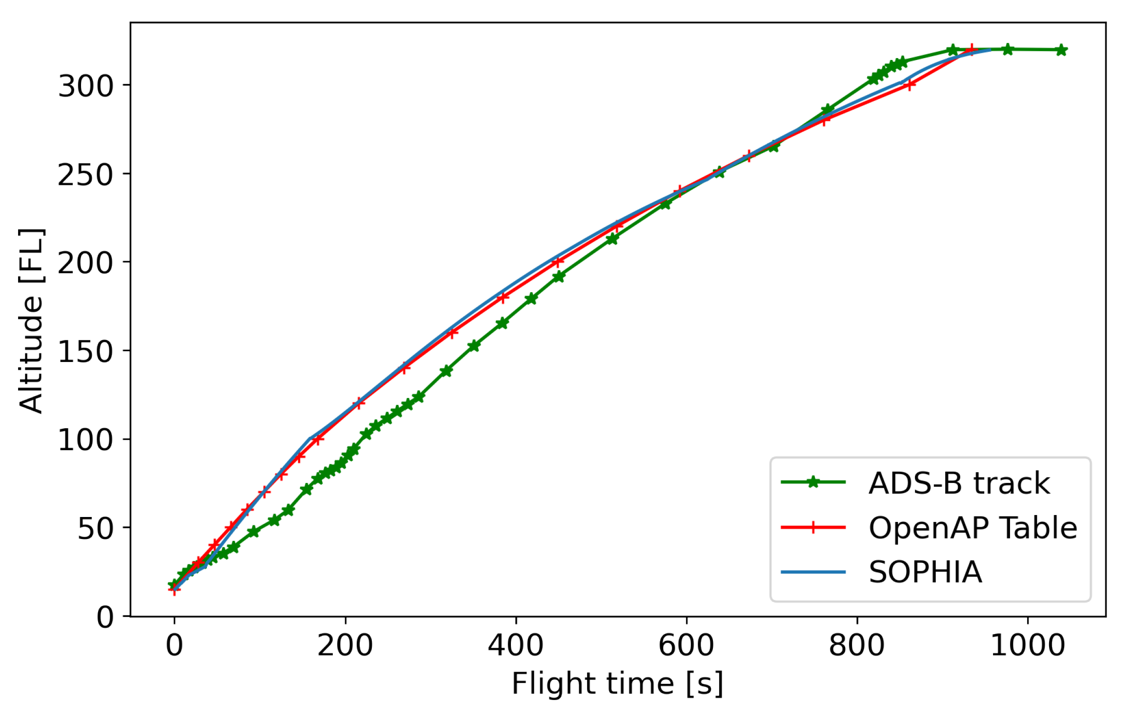
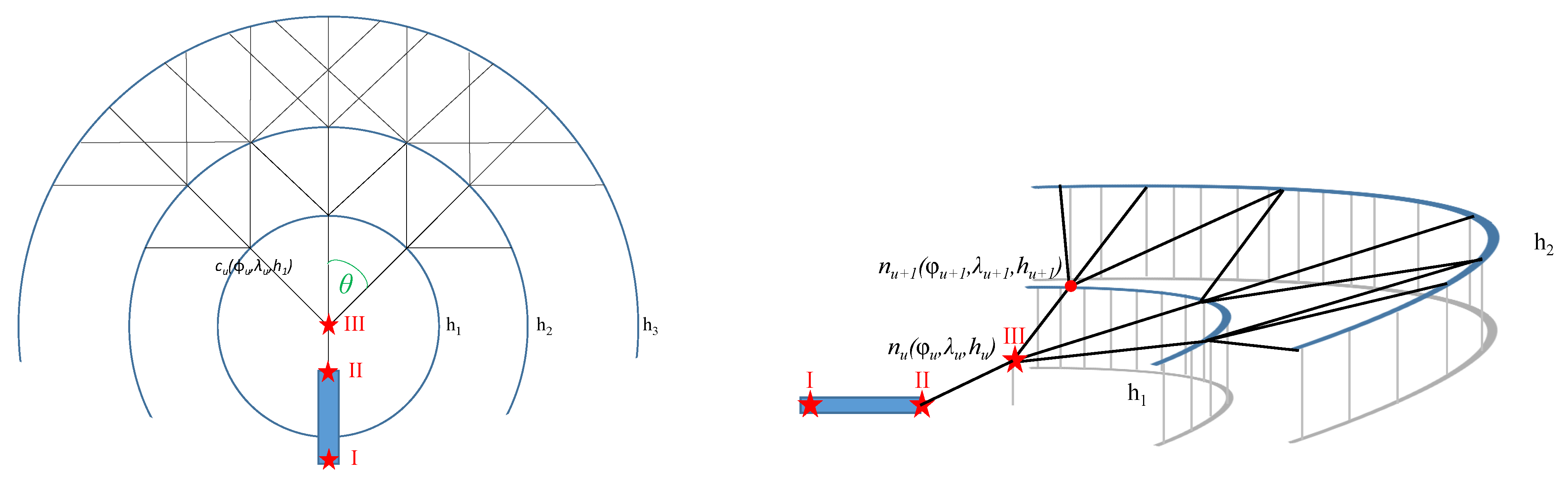
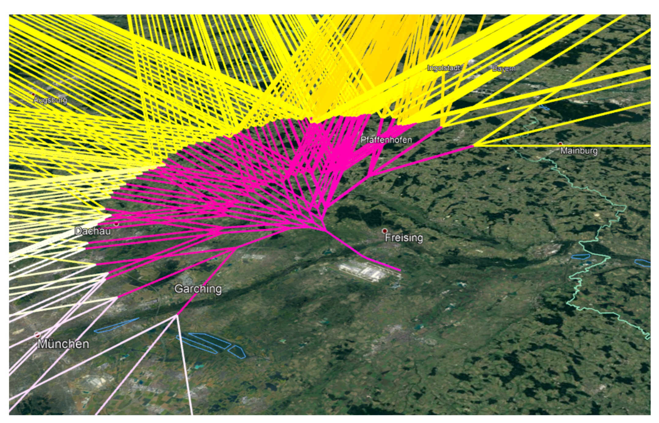
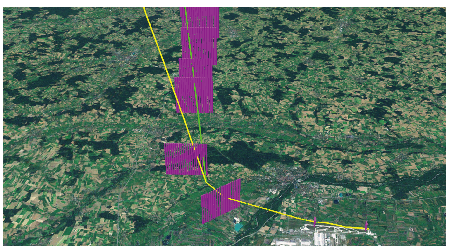
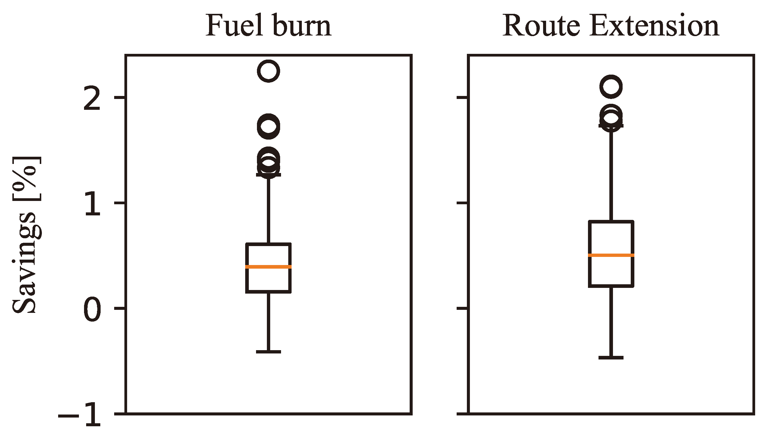
Table 1.
Difference in gate width due to wind at 10, 20, and 60 km along-track distance from runway threshold for several aircraft configurations and all freely optimized flights.
Table 1.
Difference in gate width due to wind at 10, 20, and 60 km along-track distance from runway threshold for several aircraft configurations and all freely optimized flights.
| Aircraft | 10 km | 20 km | 60 km | |||
|---|---|---|---|---|---|---|
| Mean | STD | Mean | STD | Mean | STD | |
| [m] | [m] | [m] | [m] | [m] | [m] | |
| A320 | 2088 | 1822 | 6533 | 5593 | 13,156 | 10,993 |
| B737 | 804 | 679 | 1900 | 1634 | 3784 | 3369 |
| B777 | 821 | 709 | 2247 | 1922 | 5274 | 4286 |
Table 2.
Difference in gate height due wind at 10, 20, and 60 km along track distance from runway threshold for several aircraft configurations and all freely optimized flights.
Table 2.
Difference in gate height due wind at 10, 20, and 60 km along track distance from runway threshold for several aircraft configurations and all freely optimized flights.
| Aircraft | Gross Mass [kg] | 10 km | 20 km | 60 km | |||
|---|---|---|---|---|---|---|---|
| Mean | STD | Mean | STD | Mean | STD | ||
| [m] | [m] | [m] | [m] | [m] | [m] | ||
| A320 | 39,000 | 355 | 69 | 490 | 110 | 197 | 52 |
| 58,000 | 204 | 40 | 246 | 52 | 336 | 86 | |
| 77,000 | 183 | 37 | 226 | 46 | 227 | 57 | |
| B737 | 41,500 | 395 | 77 | 429 | 96 | 196 | 52 |
| 60,200 | 221 | 44 | 214 | 45 | 328 | 85 | |
| 79,000 | 185 | 38 | 221 | 45 | 344 | 92 | |
| B777 | 145,000 | 320 | 61 | 511 | 111 | 215 | 57 |
| 246,500 | 157 | 32 | 236 | 49 | 727 | 207 | |
| 347,500 | 83 | 16 | 188 | 37 | 268 | 69 | |
Table 3.
Dimension of departure funnels and grid point spacing per gate from the ADS-B data and optimized flights.
Table 3.
Dimension of departure funnels and grid point spacing per gate from the ADS-B data and optimized flights.
| Percentile | Gates of ADS-B Funnels | Gates of Optimized Funnels | |||
|---|---|---|---|---|---|
| Size | Spacing | Size | Spacing | ||
| [m] | [m] | [m] | [m] | ||
| Width | 0.05 | 2112 | 106 | 1874 | 94 |
| 0.5 | 4793 | 240 | 10,556 | 528 | |
| 0.95 | 7542 | 377 | 19,797 | 989 | |
| Height | 0.05 | 1367 | 34 | 434 | 11 |
| 0.5 | 2946 | 73 | 1719 | 43 | |
| 0.95 | 4612 | 115 | 3558 | 89 | |
Publisher’s Note: MDPI stays neutral with regard to jurisdictional claims in published maps and institutional affiliations. |
© 2022 by the authors. Licensee MDPI, Basel, Switzerland. This article is an open access article distributed under the terms and conditions of the Creative Commons Attribution (CC BY) license (https://creativecommons.org/licenses/by/4.0/).
Share and Cite
MDPI and ACS Style
Lindner, M.; Zeh, T.; Braßel, H.; Rosenow, J.; Fricke, H. Traffic Flow Funnels Based on Aircraft Performance for Optimized Departure Procedures. Future Transp. 2022, 2, 711-733. https://doi.org/10.3390/futuretransp2030040
AMA Style
Lindner M, Zeh T, Braßel H, Rosenow J, Fricke H. Traffic Flow Funnels Based on Aircraft Performance for Optimized Departure Procedures. Future Transportation. 2022; 2(3):711-733. https://doi.org/10.3390/futuretransp2030040
Chicago/Turabian StyleLindner, Martin, Thomas Zeh, Hannes Braßel, Judith Rosenow, and Hartmut Fricke. 2022. "Traffic Flow Funnels Based on Aircraft Performance for Optimized Departure Procedures" Future Transportation 2, no. 3: 711-733. https://doi.org/10.3390/futuretransp2030040